Linear mixed models in practice: When ANCOVA is enough and when you really need random effects
In our lab this week, a recurring question came up again: When should we use linear mixed models, how do they differ from “classical” approaches such as ANOVA or ANCOVA, and how should the results be interpreted in practice? This post is a walkthrough that hopefully clarifies the conceptual differences and shows, why many experimental designs in neuroscience (and other fields) should be considered hierarchical and thus call for mixed models.
) Fixed, mixed, and random effects influence linear regression models. Linear mixed models explicitly model correlations in hierarchical or grouped data via random effects. They extend standard linear regression by adding random intercepts and slopes to capture variability between groups or subjects. In cases, your data are clustered or correlated (e.g., repeated measures, nested designs), LMMs provide a flexible framework to account for these dependencies, improving inference and interpretability. Source: Wikimedia Commons (license: CC BY-SA 4.0)
Fixed, mixed, and random effects influence linear regression models. Linear mixed models explicitly model correlations in hierarchical or grouped data via random effects. They extend standard linear regression by adding random intercepts and slopes to capture variability between groups or subjects. In cases, your data are clustered or correlated (e.g., repeated measures, nested designs), LMMs provide a flexible framework to account for these dependencies, improving inference and interpretability. Source: Wikimedia Commons (license: CC BY-SA 4.0)
Linear mixed models (LMMs), also called linear mixed effects models, extend classical linear regression and ANOVA by explicitly representing hierarchical dependence structures. They are the default tool when observations are grouped or repeated, and thus not independent. Typical examples are
- repeated measurements per subject,
- multiple neurons per animal,
- multiple sessions per day, or
- trials nested within sessions nested within animals.
In all these cases, “ordinary” regression treats correlated observations as if they were independent and can therefore deliver misleading standard errors, p values, and effect estimates.
The central idea of mixed models is simple: Separate the effect structure into a part that is assumed to be shared across the whole population and a part that captures systematic variation between groups.
Why and when LMM instead of a t test, ANOVA, or ANCOVA
Classical tests such as the t test or ANOVA assume independent observations, or they allow dependence only under very restrictive covariance assumptions and balanced designs. Real experiments, especially in neuroscience, rarely satisfy these assumptions. Typically, measurements within the same animal, neuron, day, or session are correlated, and the number of observations per unit is often unequal.
LMMs are preferable in these situations because they represent dependence via random effects rather than by forcing you into ad hoc aggregation, dropping data to balance designs, or ignoring hierarchy altogether. They can handle unbalanced designs, incorporate continuous covariates naturally, and model individual variability in effects through random slopes. Repeated measures ANOVA can be understood as a special case of an LMM with a strongly constrained covariance structure. The t test is another special case of a linear model in which the predictor is binary and there are no random effects.
A useful practical summary is: If your data are clustered or repeated and you care about inference at the population level, treat the grouping explicitly. Sometimes fixed effects ANCOVA is sufficient, sometimes it is not. The distinction becomes sharp when
- the number of groups grows,
- the number of observations per group becomes small,
- the design becomes unbalanced, or
- you need to generalize beyond the observed groups.
The core model in equations
A linear mixed model consists of two components:
- fixed effects: Effects of interest that are systematically estimated (e.g., stimulus condition, time, group).
- random effects: Random deviations of individual groups/individuals from the population (e.g., different baselines per person, different slopes per neuron).
Let’s look at this mathematically. An LMM is typically written as
\[\begin{align} \mathbf{y} = \mathbf{X}\boldsymbol{\beta} + \mathbf{Z}\mathbf{b} + \boldsymbol{\varepsilon}. \end{align}\]Here, $\mathbf{y}\in\mathbb{R}^n$ is the vector of observed responses, $\mathbf{X}$ is the fixed effect design matrix, $\boldsymbol{\beta}$ are the fixed effect coefficients, $\mathbf{Z}$ is the random effect design matrix, $\mathbf{b}$ are the group specific random effect coefficients, and $\boldsymbol{\varepsilon}$ are residuals.
The assumptions are
\[\begin{align} \mathbf{b}\sim\mathcal{N}(\mathbf{0},\mathbf{G}), \\ \boldsymbol{\varepsilon}\sim\mathcal{N}(\mathbf{0},\mathbf{R}), \end{align}\]and $\mathbf{b}$ and $\boldsymbol{\varepsilon}$ are independent. Therefore
\[\begin{align} \mathbf{y}\sim\mathcal{N}\!\left(\mathbf{X}\boldsymbol{\beta},\; \mathbf{Z}\mathbf{G}\mathbf{Z}^\top + \mathbf{R}\right). \end{align}\]The term $\mathbf{Z}\mathbf{G}\mathbf{Z}^\top$ is where the hierarchy lives. It induces correlations between observations that share a group identity. This is exactly what ordinary regression cannot represent.
Random intercept model
Random intercepts allow each group or subject to have its own baseline level. This is useful when subjects differ in their average response, but the effect of predictors is assumed to be the same across subjects.
For subject $i$ and observation $j$, a random intercept model reads
\[\begin{align} y_{ij} &= \beta_0 + \beta_1 x_{ij} + b_{0i} + \varepsilon_{ij}, \end{align}\]with $b_{0i}\sim\mathcal{N}(0,\sigma_0^2)$ and $\varepsilon_{ij}\sim\mathcal{N}(0,\sigma^2)$. Each subject has its own baseline shift $b_{0i}$ around the population intercept $\beta_0$.
Random intercept and random slope model
Random intercept and random slope model allow each group or subject to have its own baseline and its own sensitivity to predictors. This is useful when subjects differ not only in their average response but also in how they respond to changes in predictors.
This means, if subjects differ in their baseline and in their sensitivity to $x$, we write
\[\begin{align} y_{ij} &= \beta_0 + \beta_1 x_{ij} + b_{0i} + b_{1i}x_{ij} + \varepsilon_{ij}, \end{align}\]with
\[\begin{align}\begin{pmatrix} b_{0i} \\ b_{1i}\end{pmatrix}&\sim\mathcal{N}\!\left(\begin{pmatrix}0\\0\end{pmatrix},\begin{pmatrix}\sigma_0^2 & \rho\sigma_0\sigma_1 \\ \rho\sigma_0\sigma_1 & \sigma_1^2\end{pmatrix}\right). \end{align}\]The correlation parameter $\rho$ matters in practice. It captures whether higher baseline subjects also tend to have steeper or flatter slopes.
BLUPs
The group specific random effect estimates $\hat{\mathbf{b}}_i$ that are often printed in software output are conditional estimates given the data. In the classical terminology, they are called Best Linear Unbiased Predictors (BLUPs). They should not be interpreted as independent fixed parameters but as shrunken estimates under a hierarchical prior implied by $\mathbf{b}\sim\mathcal{N}(0,\mathbf{G})$.
General interpretation of results
Fixed effects are population level parameters. They answer questions such as: Does stimulus strength increase the response on average, across animals. In typical mixed model output (e.g., statsmodels in Python which we will use in our example below), these are the coefficients in the top part of the table, typically accompanied by a standard error and a Wald statistic. In a random intercept and slope model, the fixed effects define the population line, the average intercept $\beta_0$ and average slope $\beta_1$.
Random effects describe between group variability and thereby the induced dependence structure. Their variances and covariances are variance components. They answer questions such as: How much do animals differ in baseline response, how much do they differ in stimulus sensitivity, and are those two differences correlated. The group specific random effect estimates that are often printed are conditional estimates given the data. In the classical terminology, they are BLUPs. They should not be interpreted as independent fixed parameters but as shrunken estimates under a hierarchical prior implied by $\mathbf{b}\sim\mathcal{N}(0,\mathbf{G})$.
Model diagnostics should address whether residuals are compatible with the assumed Gaussian noise model, whether variance is roughly constant across fitted values, whether random effects are plausible, whether the optimizer converged, and whether the random effect structure is overparameterized. “Singular” fits or near zero variance components indicate that the model is too complex for the information content in the data. Thus, tools to assess model fit and assumptions are:
- Residuals vs. Fits plots (first check)
- QQ-plots (also show residuals, but also random effects)
- Normality of Random Effects (BLUPs)
- Singular fits (zero variance components)
Numerical example in Python
In order to illustrate the concepts above, we implement a small didactic pipeline in Python. The structure and the diagnostic visualizations are adapted from Edouard Duchesnayꜛ’s excellent LMM tutorialꜛ. The main change is that the example dataset is framed in neuroscience terms, i.e., we simulate some artificial neural responses with stimulus strength as a continuous predictor and neural response as the dependent variable. Many thanks to Edouard Duchesnay for making this material openly available and for setting such a high standard for didactic explanations!
We will proceed as follows. We first simulate grouped data, inspect raw structure, and then fit a sequence of models that incrementally represent the hierarchy:
- global OLS,
- ANCOVA with group intercepts,
- aggregation and two stage approaches, and
- mixed models with random intercepts and random intercepts plus slopes.
We then compare fitted lines and residual diagnostics and finally highlight one of the most important conceptual differences between ANCOVA with group specific slopes and LMMs: Shrinkage.
Toy dataset generation
As described above, we simulate a dataset with multiple animals, each contributing multiple observations at different stimulus strengths.
The simulator function defined below draws a set of animals and assigns each animal a random intercept and a random slope around population parameters $\beta_0$ and $\beta_1$. Observations are then generated at discrete stimulus strengths and corrupted by Gaussian noise. This produces exactly the kind of clustered structure one encounters in practice: Data points are not independent because points from the same animal share latent offsets.
Let’s implement this in code. We begin by importing the necessary libraries and setting some general plotting aesthetics for the entire script:
import os
import numpy as np
import pandas as pd
import matplotlib.pyplot as plt
import seaborn as sns
import itertools
import scipy.stats as spstats
import statsmodels.api as sm
import statsmodels.formula.api as smf

# remove spines right and top for better aesthetics:
plt.rcParams['axes.spines.right'] = False
plt.rcParams['axes.spines.top'] = False
plt.rcParams['axes.spines.left'] = False
plt.rcParams['axes.spines.bottom'] = False
plt.rcParams.update({'font.size': 12})
Here is the simulator function:
def simulate_animal_data(
    seed=0,
    n_animals=6,
    n_obs_per_animal=40,
    beta0=8.0,             # population intercept
    beta1=0.25,            # population slope for x
    sigma_animal_intercept=2.5,
    sigma_animal_slope=0.12,
    sigma_noise=1.0):
    rng = np.random.default_rng(seed)
    animals = [f"subj_{i}" for i in range(n_animals)]

    # animal random intercepts and slopes:
    b0 = rng.normal(0.0, sigma_animal_intercept, size=n_animals)
    b1 = rng.normal(0.0, sigma_animal_slope, size=n_animals)

    rows = []
    for i, a in enumerate(animals):
        # choose a plausible x distribution:
        # e.g. stimulus strength 0..10
        x = rng.integers(0, 11, size=n_obs_per_animal).astype(float)

        # conditional mean with animal specific intercept and slope
        mu = (beta0 + b0[i]) + (beta1 + b1[i]) * x
        y = mu + rng.normal(0.0, sigma_noise, size=n_obs_per_animal)

        for xx, yy in zip(x, y):
            rows.append({"animal": a, "x": xx, "y": yy})

    return pd.DataFrame(rows)
We generate a dataset with three animals, each contributing 40 observations at different stimulus strengths. The population intercept is set to 8.0, the population slope to 0.25, and we specify standard deviations for animal-specific intercepts and slopes as well as observation noise:
outpath = "llm_results"
os.makedirs(outpath, exist_ok=True)
df = simulate_animal_data(seed=41,
                          n_animals=3,
                          n_obs_per_animal=40,
                          beta0=8.0,
                          beta1=0.25,
                          sigma_animal_intercept=2.5,
                          sigma_animal_slope=0.12,
                          sigma_noise=1.0)
Let’s visualize the raw data, color coded by animal:
plt.figure(figsize=(6.5, 4))
for a, g in df.groupby("animal"):
    plt.scatter(g["x"], g["y"], s=35, alpha=0.8, label=a, lw=0)
plt.xlabel("x: stimulus strength (=continuous predictor)")
plt.ylabel("y: neural response (=dependent variable)")
plt.title("Raw data, grouped by animal")
plt.legend(frameon=False, bbox_to_anchor=(1.0, 1), loc='upper left')
plt.tight_layout()
plt.savefig(os.path.join(outpath, "raw_data_by_animal.png"), dpi=300)
plt.close()
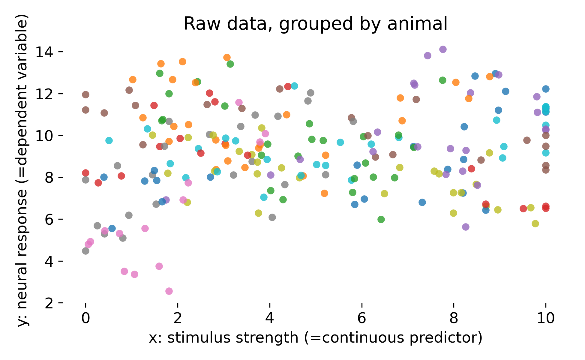
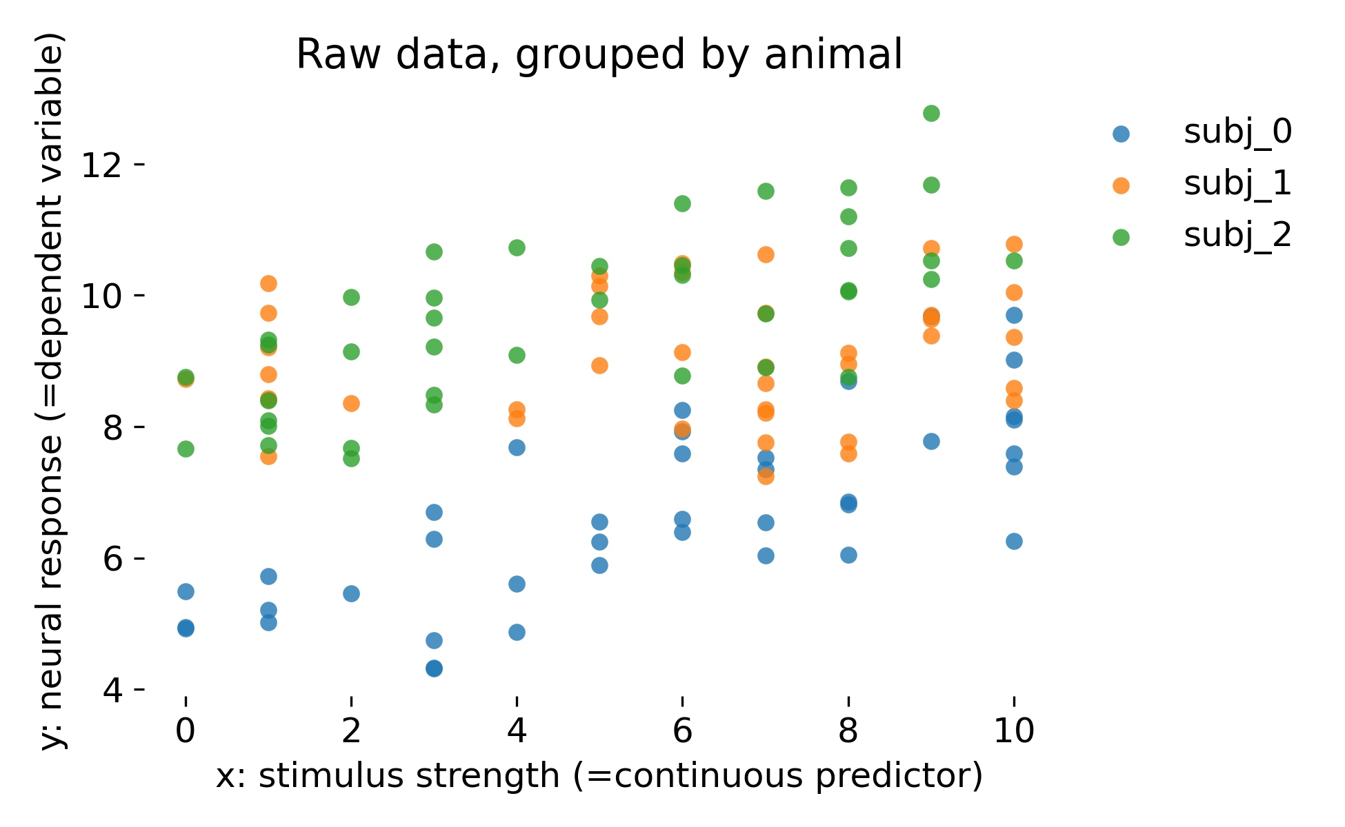 Raw simulated dataset grouped by animal. Each point is a single observation with stimulus strength $x$ and response $y$. Colors indicate animals, illustrating that animals differ both in baseline response and in the apparent dependence on stimulus strength.
The key feature in our dataset is that points within an animal are more similar to each other than points across animals. This is a direct violation of the independence assumption of ordinary least squares. A global regression line cannot represent the fact that each animal occupies its own band in response space (as we will see in the next section). Any method that treats all points as independent risks overstating certainty because it counts within animal variation as independent evidence.
Helper functions for diagnostics
Before we continue with model fitting, we define two helper functions for plotting diagnostic figures. The first function creates QQ plots of residuals, the second function creates residuals vs. fits plots and residual distributions, optionally grouped by animal.
The diagnostic visualizations serve two roles. The QQ plot checks whether residuals are compatible with a Gaussian distribution under the fitted model. The three panel residual plot provides a quick view of heteroscedasticity or systematic patterns in residuals, the overall residual distribution, and whether residual distributions differ across groups. These are not sufficient conditions for model correctness, but they are necessary checks that should be routine.
def plot_qq_diagnostics(resid, fitted, groups, title_prefix, outpath=None):
    fig, ax = plt.subplots(figsize=(4, 4))
    sm.qqplot(resid, line="45", fit=True, ax=ax, alpha=0.7, lw=0)
    ax.set_title(f"{title_prefix}:\nQQ plot of residuals")
    plt.tight_layout()
    if outpath is not None:
        plt.savefig(os.path.join(outpath, f"{title_prefix}_qqplot.png"), dpi=300)
        plt.close()
    else:
        plt.show()
def plot_residual_diagnostics(residual, prediction, group=None, group_boxplot=False,
                      title_prefix="", outpath=None, fname_prefix=""):
    diag_df = pd.DataFrame(dict(prediction=np.asarray(prediction), residual=np.asarray(residual)))
    if group is not None:
        diag_df["group"] = np.asarray(group)

        fig, axes = plt.subplots(1, 3, figsize=(7, 3.5), sharey=True)

        sns.scatterplot(
            x="prediction", y="residual", hue="group", data=diag_df,
            ax=axes[0], s=35, alpha=0.85, legend=False
        )
        axes[0].axhline(0.0, linewidth=1.0)
        axes[0].set_title("Residuals vs pred")

        sns.kdeplot(y="residual", data=diag_df, fill=True, ax=axes[1])
        axes[1].set_title("Residuals")

        if group_boxplot:
            sns.boxplot(y="residual", x="group", data=diag_df, ax=axes[2])
            axes[2].set_title("Residuals by group")
        else:
            sns.kdeplot(y="residual", hue="group", data=diag_df, fill=True, ax=axes[2])
            axes[2].set_title("Residuals by group")

        # if group/animal size is >4, don't show legend:
        if diag_df["group"].nunique() <= 4:
            # ensure legend is visible and tidy
            leg = axes[2].get_legend()
            if leg is None:
                axes[2].legend(title="group", frameon=False)
            else:
                leg.set_frame_on(False)
        else:
            # remove legend for many groups
            leg = axes[2].get_legend()
            if leg is not None:
                leg.remove()

        if title_prefix:
            fig.suptitle(title_prefix)
        plt.tight_layout()

        if outpath is not None:
            os.makedirs(outpath, exist_ok=True)
            fn = f"{fname_prefix}_lm_diagnosis.png" if fname_prefix else "lm_diagnosis.png"
            plt.savefig(os.path.join(outpath, fn), dpi=300)
            plt.close()
        else:
            plt.show()

    else:
        fig, axes = plt.subplots(1, 2, figsize=(7, 3.5), sharey=True)
        sns.scatterplot(x="prediction", y="residual", data=diag_df, ax=axes[0], s=35, alpha=0.85)
        axes[0].axhline(0.0, linewidth=1.0)
        axes[0].set_title("Residuals vs pred")

        sns.kdeplot(y="residual", data=diag_df, fill=True, ax=axes[1])
        axes[1].set_title("Residuals")

        if title_prefix:
            fig.suptitle(title_prefix)
        plt.tight_layout()

        if outpath is not None:
            os.makedirs(outpath, exist_ok=True)
            fn = f"{fname_prefix}_lm_diagnosis.png" if fname_prefix else "lm_diagnosis.png"
            plt.savefig(os.path.join(outpath, fn), dpi=300)
            plt.close()
        else:
            plt.show()
We will use these functions repeatedly below to assess model fit.
Global OLS ignoring grouping
Our first model is a global ordinary least squares (OLS). The global OLS slope is an average trend across all points, but it implicitly assumes that each point contributes independent information. In clustered data, this is false. Visually, the line cuts through the cloud (see plot below), but it does not represent the animal specific structure. Inferentially, the main danger is not that the slope estimate is always wrong. The more severe problem is that standard errors and p values can become overly optimistic because within animal correlation reduces the effective sample size. Global OLS therefore answers the wrong question: It tests whether a population trend exists if all points were independent, rather than whether a population trend exists given correlated repeated measurements.
Let’s fit the global OLS model and inspect the results:
lm_global = smf.ols("y ~ x", data=df).fit()
print("\nGlobal OLS: y ~ x")
print(lm_global.summary().tables[1])
Here is the print output of the model summary:
Global OLS: y ~ x
==============================================================================
                 coef    std err          t      P>|t|      [0.025      0.975]
------------------------------------------------------------------------------
Intercept      7.4405      0.310     24.035      0.000       6.827       8.054
x              0.1898      0.050      3.832      0.000       0.092       0.288
==============================================================================
The print out shows a typical OLS summary with coefficient estimates, standard errors, t statistics, and p values. The estimated slope is 0.1898 with a standard error of 0.050, leading to a t statistic of 3.832 and a highly significant p value. However, as we will see in the diagnostics below, these numbers are misleading because the model ignores the grouping structure.
Now let’s investigate the plots:
plot_qq_diagnostics(
    resid=lm_global.resid.to_numpy(),
    fitted=lm_global.fittedvalues.to_numpy(),
    groups=df["animal"].to_numpy(),
    title_prefix="Global_OLS",
    outpath=outpath)

# global fit plot:
legend_on = df["animal"].nunique() <= 6
fig, ax = plt.subplots(figsize=(6.5, 4))
# scatter by animal:
sns.scatterplot(x="x", y="y", hue="animal", data=df, s=35, alpha=0.8, lw=0,
    legend=legend_on,ax=ax)
# global OLS line
xline = np.linspace(df["x"].min(), df["x"].max(), 200)
yline = lm_global.params["Intercept"] + lm_global.params["x"] * xline
ax.plot(xline, yline, color="k", linewidth=2.0)
ax.set_xlabel("x: stimulus strength")
ax.set_ylabel("y: neural response")
ax.set_title("Global OLS fit (ignores grouping)")
# remove left and bottom spines for aesthetics:
ax.spines["bottom"].set_visible(False)
ax.spines["left"].set_visible(False)
if legend_on:
    ax.legend(frameon=False, bbox_to_anchor=(1.00, 1), loc="upper left")
else:
    ax.get_legend().remove()
plt.tight_layout()
plt.savefig(os.path.join(outpath, "Global_OLS_fit.png"), dpi=300)
plt.close()

plot_residual_diagnostics(
    residual=lm_global.resid,
    prediction=lm_global.predict(df),
    group=df["animal"],
    title_prefix="Global OLS",
    outpath=outpath,
    fname_prefix="Global_OLS")
The first plot shows the global OLS fit. As expected, the single regression line cuts through the cloud of points but does not represent the animal specific structure:
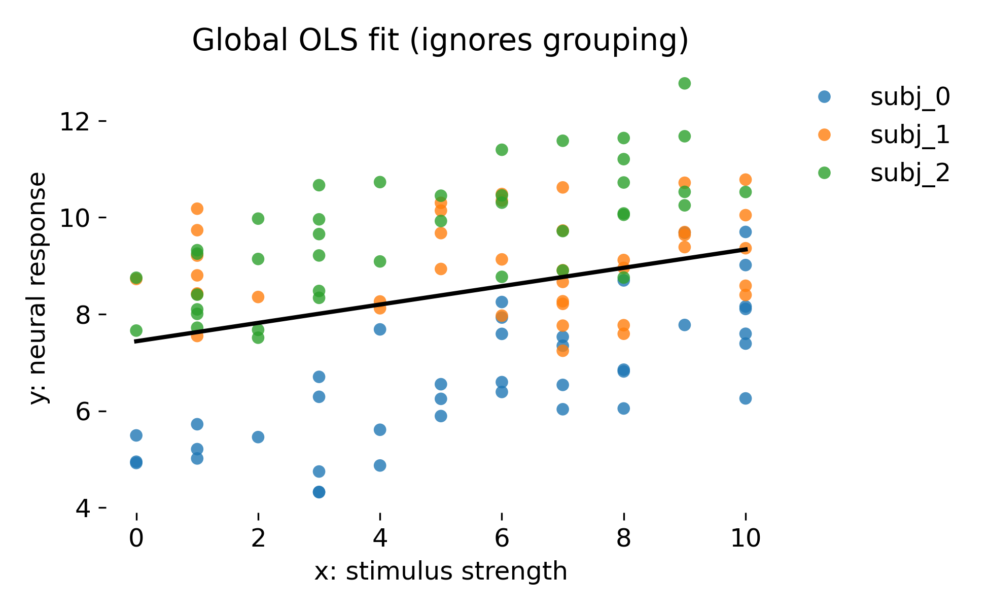 Global OLS fit that ignores grouping. The black line is the single regression line fitted to all observations. Colors denote animals, which are not represented in the model.
Here is the QQ plot of residuals:
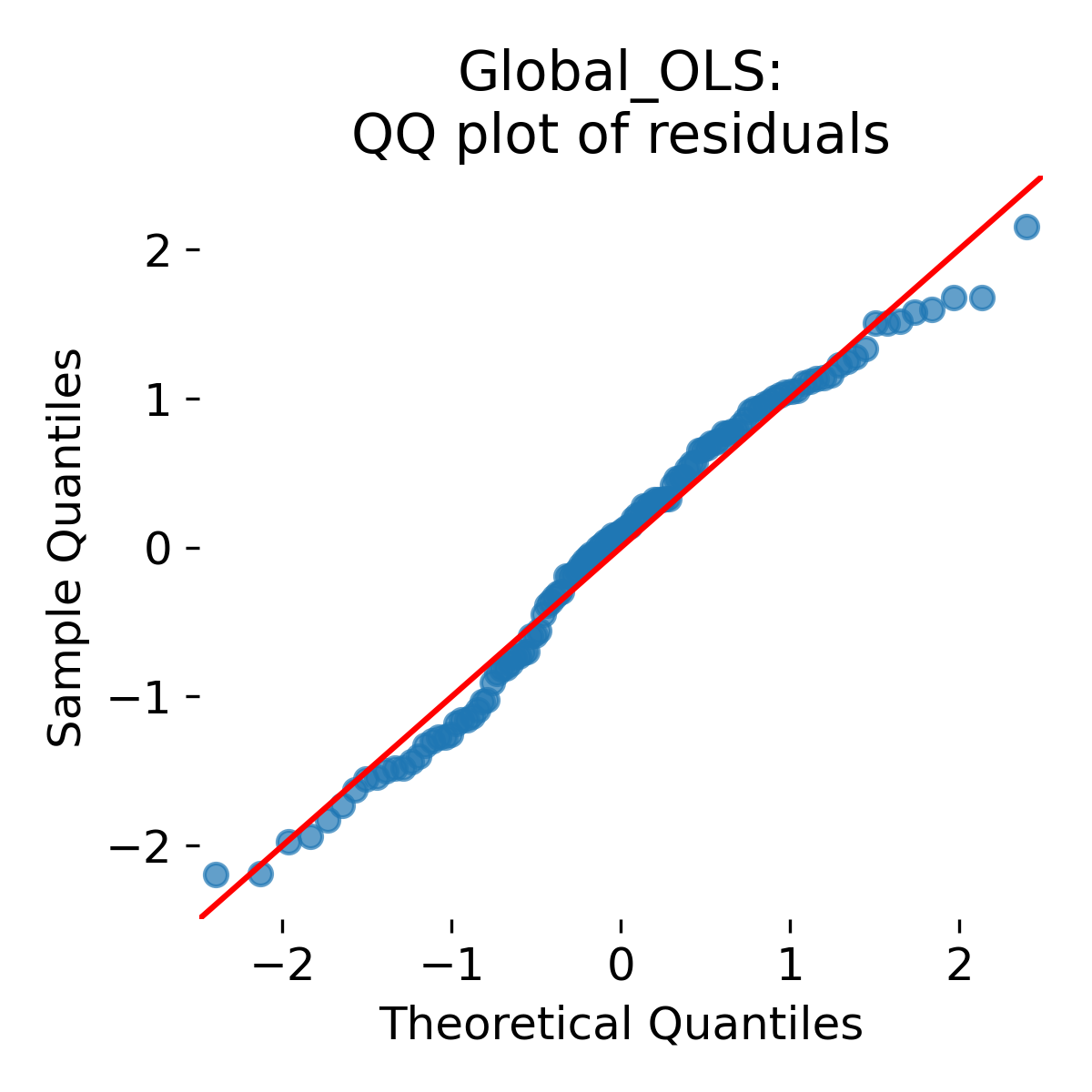
QQ plot of global OLS residuals. Points close to the diagonal indicate approximate normality of residuals under the model, while systematic deviations indicate heavier tails or skewness.
It shows almost perfect agreement with the diagonal, indicating that residuals are approximately Gaussian under the model. This is expected because the data were generated from a Gaussian model. However, this does not mean that the model is valid for inference because it ignores the grouping structure. Independence violations are not diagnosed by a QQ plot. A model can have approximately Gaussian residuals and still be statistically invalid for inference because it misrepresents the covariance structure.
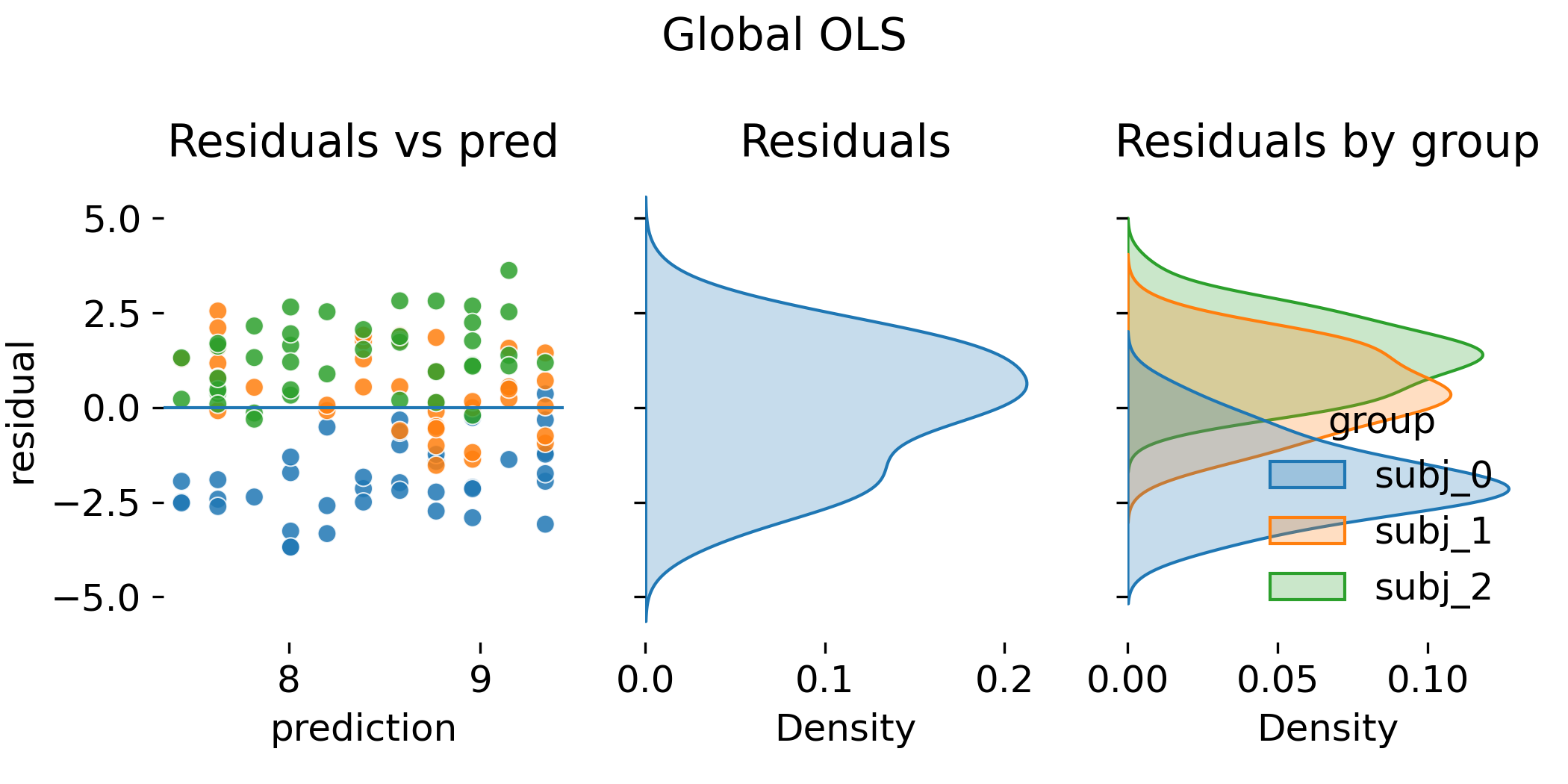
This is confirmed by the residual diagnostics:
 QQ plot of global OLS residuals. Points close to the diagonal indicate approximate normality of residuals under the model, while systematic deviations indicate heavier tails or skewness.
The per animal residual densities indicate systematic shifts that the model cannot absorb. Conceptually, the model tries to explain between animal variation as residual noise. This inflates the residual variance and distorts standard errors. The plot shows why “looking only at the residual cloud” is insufficient. The fitted values already encode the wrong dependence structure.
Before we continue: As we fit several models, we define a small utility function to track a small set of comparable summary quantities: RMSE as a crude measure of predictive error, the estimated coefficient for $x$, and its test statistic and p value as reported by statsmodels. This table is not meant to be a formal model selection device. Its purpose is to show how effect estimates and their uncertainty change when we change the model’s representation of hierarchy:
def rmse_coef_tstat_pval(mod, var: str):
    resid = np.asarray(mod.resid)
    sse = float(np.sum(resid ** 2))
    df_resid = float(getattr(mod, "df_resid", len(resid) - 1))

    rmse = np.sqrt(sse / df_resid)

    coef = float(mod.params[var])

    # OLS: tvalues, MixedLM: zvalues
    if hasattr(mod, "tvalues") and (var in getattr(mod, "tvalues", {})):
        stat = float(mod.tvalues[var])
    elif hasattr(mod, "tvalues") and isinstance(mod.tvalues, (pd.Series, np.ndarray)):
        stat = float(mod.tvalues[var])
    else:
        # MixedLMResults: use z-values
        stat = float(mod.tvalues[var]) if hasattr(mod, "tvalues") else float(mod.params[var] / mod.bse[var])

    pval = float(mod.pvalues[var])

    return rmse, coef, stat, pval
# create and store first summary row:
rmse, coef, stat, pval = rmse_coef_tstat_pval(lm_global, "x")
results = pd.DataFrame(columns=["Model", "RMSE", "Coef_x", "Stat_x", "Pval_x"])
results.loc[len(results)] = ["OLS global (biased SE)", rmse, coef, stat, pval]
ANCOVA with animal as fixed intercept shifts
Next, we fit an ANCOVA model with animal as a categorical fixed effect. This model allows each animal to have its own intercept shift, but it assumes a common slope across animals. This is equivalent to fitting separate intercepts per animal while constraining the slope to be the same.
def plot_ancova_oneslope_grpintercept(x, y, group, df, model, outpath=None, fname="ancova_oneslope_grpintercept.png"):
    """
    ANCOVA: one common slope, group specific fixed intercept shifts.

    Model form: y ~ x + C(group)
    Plot: scatter by group + black lines with same slope, shifted intercept.
    """
    legend_on = True if df[group].nunique() <= 6 else False
    fig, ax = plt.subplots(figsize=(6.5, 4))

    sns.scatterplot(x=x, y=y, hue=group, data=df, s=35, alpha=0.8, lw=0,
        legend=legend_on,ax=ax)

    palette = itertools.cycle(sns.color_palette())
    x_jitter = -0.2

    base_intercept = float(model.params["Intercept"])
    slope = float(model.params[x])

    for group_lab, group_df in df.groupby(group):
        x_ = group_df[x].to_numpy()
        color = next(palette)

        # fixed intercept shift for this group, reference group has 0 shift
        key = f"C({group})[T.{group_lab}]"
        group_offset = float(model.params[key]) if key in model.params else 0.0

        y_pred = base_intercept + slope * x_ + group_offset

        # draw the common-slope line for this group
        order = np.argsort(x_)
        ax.plot(x_[order], y_pred[order], color="k", linewidth=2.0)

        # arrow indicating the intercept shift
        ax.arrow(0 + x_jitter, base_intercept, 0, group_offset,
                 head_width=0.25, length_includes_head=True, color=color)
        x_jitter += 0.2

    # deactivate legend if too many groups:
    if df[group].nunique() > 6:
        leg = ax.get_legend()
        if leg is not None:
            leg.remove()
    else:
        ax.legend(frameon=False, bbox_to_anchor=(1.00, 1), loc='upper left')

    # deactivate left and bottom spines for aesthetics:
    ax.spines['left'].set_visible(False)
    ax.spines['bottom'].set_visible(False)

    # set proper x and y labels:
    ax.set_xlabel(x + ": stimulus strength")
    ax.set_ylabel(y + ": neural response")

    ax.set_title("ANCOVA: one slope, group fixed intercepts")
    plt.tight_layout()

    if outpath is not None:
        os.makedirs(outpath, exist_ok=True)
        plt.savefig(os.path.join(outpath, fname), dpi=300)
        plt.close()
    else:
        plt.show()
ancova = smf.ols("y ~ x + C(animal)", data=df).fit()
print("\nANCOVA fixed animal intercepts: y ~ x + C(animal)")
print(ancova.summary().tables[1])
ANCOVA fixed animal intercepts: y ~ x + C(animal)
=======================================================================================
                          coef    std err          t      P>|t|      [0.025      0.975]
---------------------------------------------------------------------------------------
Intercept               5.3778      0.233     23.129      0.000       4.917       5.838
C(animal)[T.subj_1]     2.3408      0.227     10.322      0.000       1.892       2.790
C(animal)[T.subj_2]     3.2313      0.228     14.156      0.000       2.779       3.683
x                       0.2278      0.030      7.608      0.000       0.169       0.287
=======================================================================================
The table shows the estimated intercept for the reference animal (subj_0), the intercept shifts for the other animals (subj_1 and subj_2), and the common slope for $x$. All coefficients are highly significant (column P>|t|). The estimated slope is now 0.2278 with a standard error of 0.030, leading to a t statistic of 7.608. Compared to the global OLS slope of 0.1898 (standard error 0.050), the slope estimate has changed and the standard error has decreased. This reflects that the model now accounts for between animal differences in baseline.
Let’s turn to the diagnostic plots:
plot_qq_diagnostics(
    resid=ancova.resid.to_numpy(),
    fitted=ancova.fittedvalues.to_numpy(),
    groups=df["animal"].to_numpy(),
    title_prefix="ANCOVA fixed intercepts",
    outpath=outpath)

# ANCOVA one slope, fixed intercept shifts (tutorial style plot)
plot_ancova_oneslope_grpintercept(
    x="x", y="y", group="animal", df=df, model=ancova,
    outpath=outpath, fname="ANCOVA_oneslope_fixed_intercepts.png")

plot_residual_diagnostics(
    residual=ancova.resid,
    prediction=ancova.predict(df),
    group=df["animal"],
    title_prefix="ANCOVA fixed intercepts",
    outpath=outpath,
    fname_prefix="ANCOVA_fixed_intercepts")

rmse, coef, stat, pval = rmse_coef_tstat_pval(ancova, "x")
results.loc[len(results)] = ["ANCOVA fixed intercepts", rmse, coef, stat, pval]
Let’s discuss the results. Here is the ANCOVA fit with one common slope and group specific fixed intercepts:
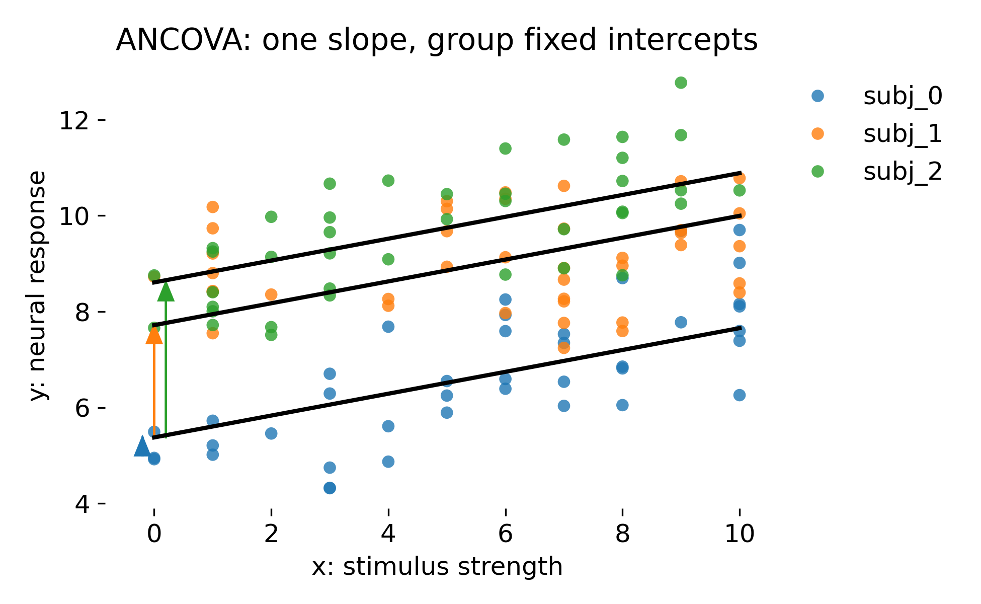 ANCOVA with one common slope and group specific fixed intercepts. Black lines have identical slope but are shifted by animal specific intercept offsets. Colored arrows illustrate the intercept shift relative to the reference intercept.
Compared to global OLS, this model acknowledges that animals differ in baseline. It effectively adds a set of animal indicator variables. This absorbs a large part of the between animal variance and therefore reduces residual variance. In this dataset, the intercept shifts are large, so this is a major improvement. However, this is still a fixed effects treatment of animals. The model estimates one intercept parameter per animal without any pooling. This can be appropriate when the animals in the dataset are the only animals of interest. In neuroscience, that is rarely the inferential goal. Usually animals are considered a random sample from a population, and one wants to generalize beyond them.
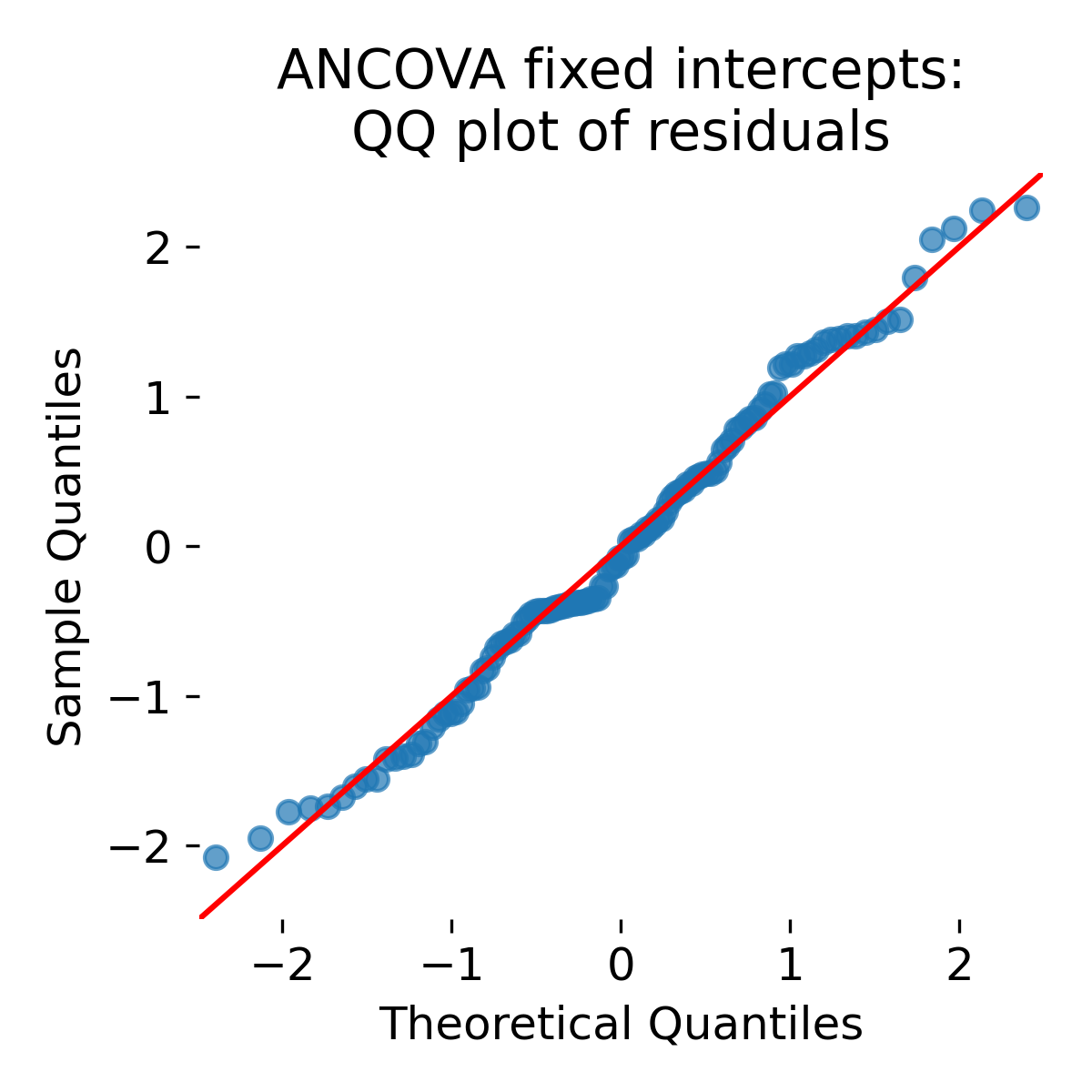
QQ plot of ANCOVA fixed intercept residuals.
Looking at the QQ plot: Residual normality can improve because between animal shifts no longer appear as unexplained noise. However, comparing to the global OLS QQ plot, there is not much change. Again, this does not decide between ANCOVA and OLS (or LMM). The key difference is how uncertainty and generalization are treated.
Let’s inspect the residual diagnostics:
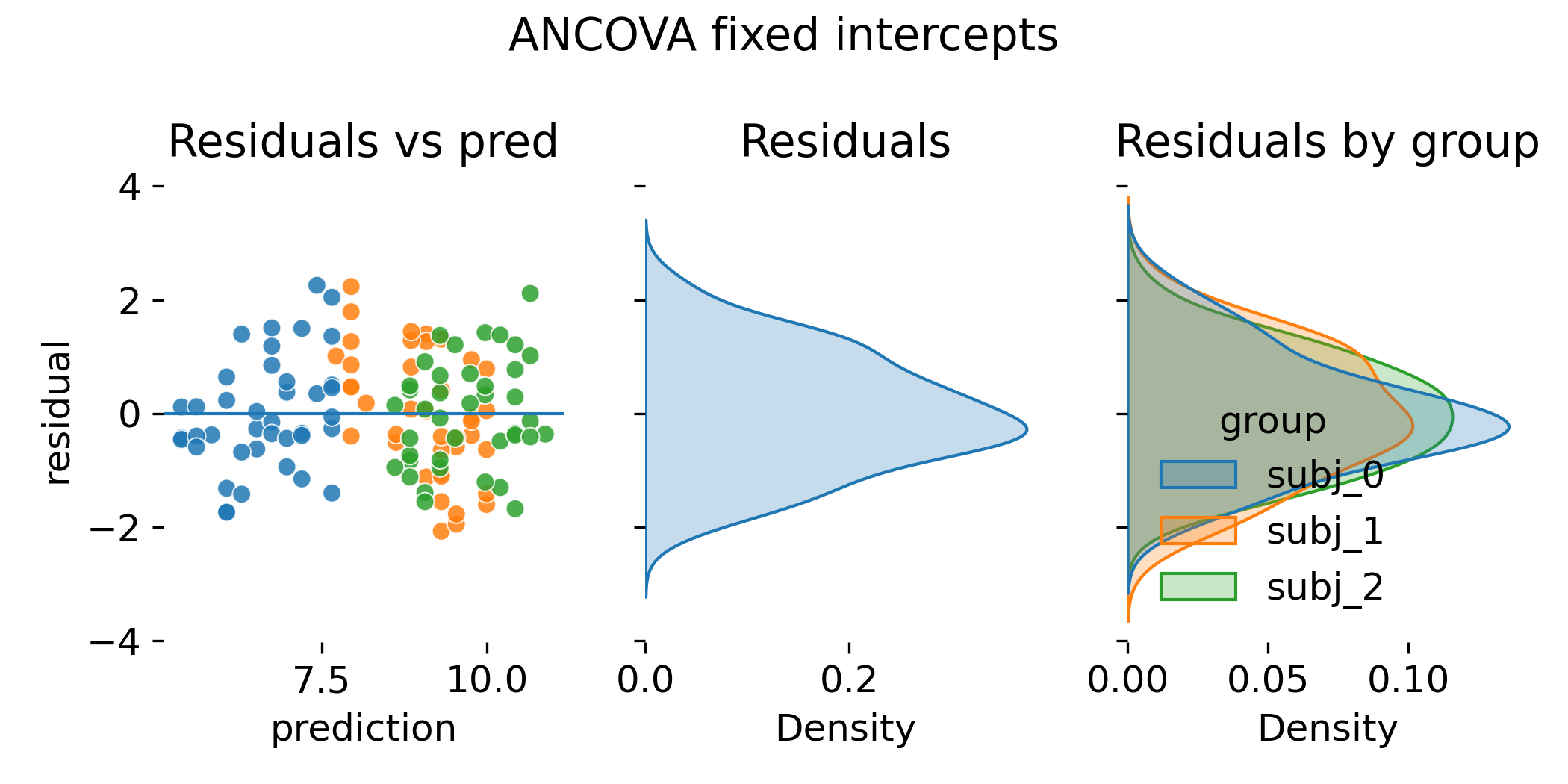 Residual diagnostics for ANCOVA with fixed intercepts.
Residual distributions across animals are now more aligned because the model explains systematic baseline differences. However, comparing this to the LMM residual diagnostics (shown later), this does not imply that both models are equivalent. Or one is better than the other. The key conceptual difference is that ANCOVA treats animal intercepts as fixed parameters to be estimated, while LMM treats them as random effects drawn from a common distribution with estimated variance. This implies shrinkage of animal specific intercept estimates toward the population mean in LMMs, while ANCOVA estimates each intercept independently. Residual diagnostics alone do not expose the central conceptual distinction. The distinction lives in how group effects are treated: Fixed parameters versus a random distribution with estimated variance.
Aggregation and why it can fail
Aggregation is sometimes suggested as a quick fix for dependence. It reduces the data to one point per animal and thereby restores independence. The price is severe: Information is thrown away and the slope becomes highly unstable because the number of data points is now the number of animals. In the toy example with only three animals, the regression on means is essentially meaningless. Even with more animals, aggregation changes the estimand: It targets the relationship between animal level means, not the within animal relationship between $x$ and $y$.
To illustrate this, we implement two aggregation based approaches. The first approach fits OLS to animal means:
agg = df.groupby("animal")[["x", "y"]].mean().reset_index()
lm_agg = smf.ols("y ~ x", data=agg).fit()
print("\nAggregation: OLS on animal means")
print(lm_agg.summary().tables[1])
Aggregation: OLS on animal means
==============================================================================
                 coef    std err          t      P>|t|      [0.025      0.975]
------------------------------------------------------------------------------
Intercept     15.4818     12.490      1.240      0.432    -143.218     174.181
x             -1.2970      2.300     -0.564      0.673     -30.519      27.925
==============================================================================
The fit output shows a highly unstable slope estimate of -1.2970 with a large standard error of 2.300, leading to a t statistic of -0.564 and a non-significant p value of 0.673. This is very different from the previous models because the aggregation approach answers a different question: It tests whether animals with higher mean stimulus strength have higher mean responses. This is not the same as testing whether within an animal, higher stimulus strength leads to higher response.
# plot aggregated points and regression
plt.figure(figsize=(6, 4))
for i, row in agg.iterrows():
    plt.scatter(row["x"], row["y"], s=120, alpha=0.9, label=row["animal"], lw=0)
xline = np.linspace(agg["x"].min(), agg["x"].max(), 100)
plt.plot(xline, lm_agg.params["Intercept"] + lm_agg.params["x"] * xline, linewidth=2.0,
         c="k", label="OLS on means")
plt.xlabel("mean x per animal")
plt.ylabel("mean y per animal")
plt.title("Aggregation level analysis")
if agg["animal"].nunique() <= 6:
    plt.legend(frameon=False, bbox_to_anchor=(1.0, 1), loc='upper left')
plt.tight_layout()
plt.savefig(os.path.join(outpath, "aggregation_level_analysis.png"), dpi=300)
plt.close()
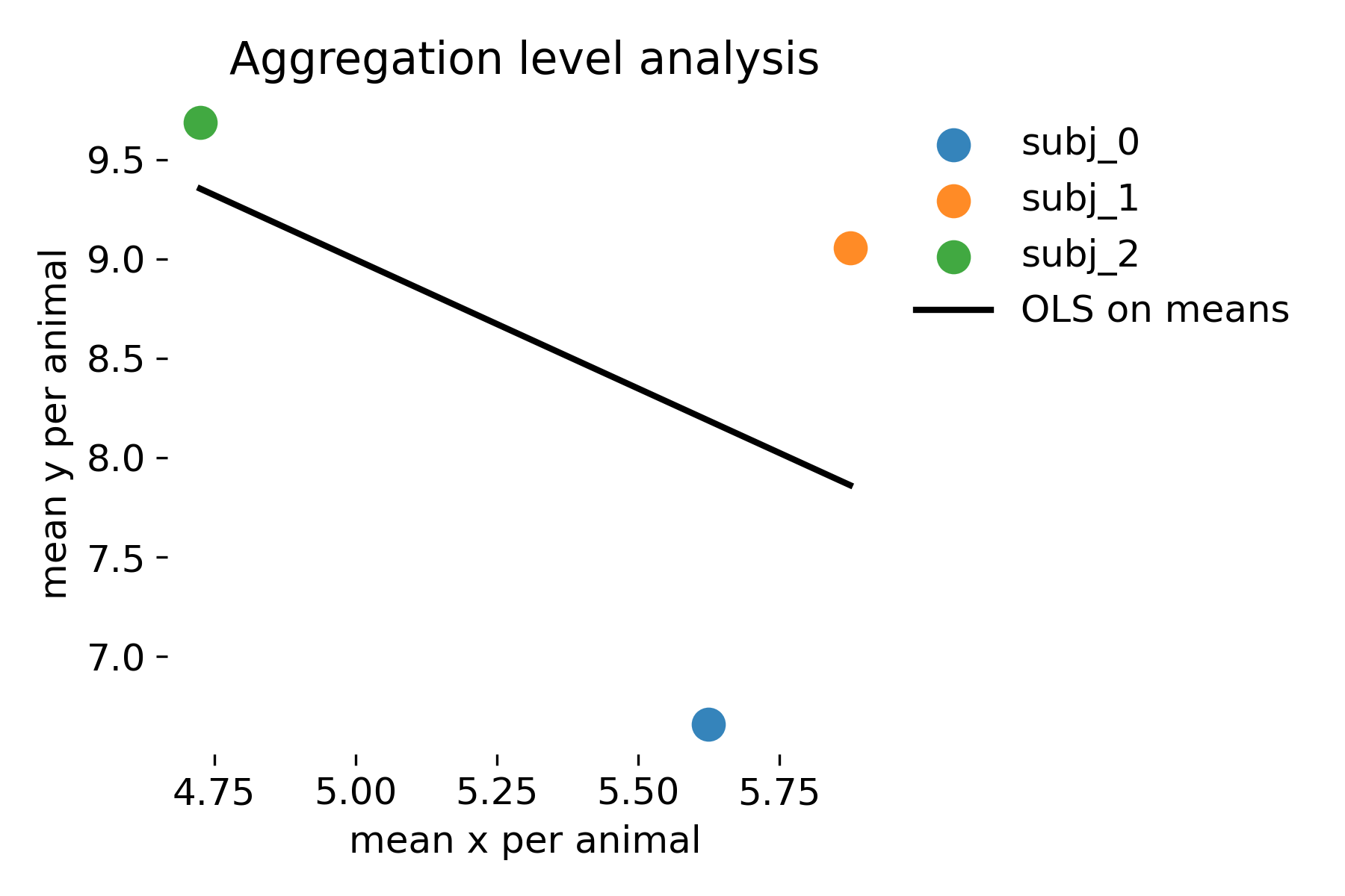 Aggregation level analysis. Each point is the mean stimulus strength and mean response per animal. The black line is an OLS fit to these animal means.
As we can see, the slope estimate is highly unstable because there are only three data points. The p value is very high, indicating no evidence for a relationship at the animal mean level. This is not surprising given the small number of animals. However, this does not imply that there is no within animal relationship between stimulus strength and response. The aggregation approach answers a different question and loses power because it discards information.
The second approach is a hierarchical two-stage approach. In the first stage, we fit separate regressions within each animal and extract the slope estimates. In the second stage, we test whether the mean slope across animals is significantly different from zero. This approach retains more information than simple aggregation because it uses within animal slopes, but it still has limitations compared to LMMs.
lv1 = []
for animal_lab, animal_df in df.groupby("animal"):
    m = smf.ols("y ~ x", data=animal_df).fit()
    lv1.append([animal_lab, float(m.params["x"])])

lv1 = pd.DataFrame(lv1, columns=["animal", "beta_x"])
lm_level2 = smf.ols("beta_x ~ 1", data=lv1).fit()

print("\nHierarchical two-stage: test mean within-animal slopes")
print(lm_level2.summary().tables[1])
Hierarchical two-stage: test mean within-animal slopes
==============================================================================
                 coef    std err          t      P>|t|      [0.025      0.975]
------------------------------------------------------------------------------
Intercept      0.2264      0.088      2.569      0.124      -0.153       0.606
==============================================================================
The table shows the estimated mean slope across animals as 0.2264 with a standard error of 0.088, leading to a t statistic of 2.569 and a p value of 0.124. This indicates some evidence for a positive relationship, but the p value is not below the conventional threshold of 0.05. This reflects the limited power of the two-stage approach, especially with only three animals.
# plot: within-animal regressions + barplot of slopes:
fig, axes = plt.subplots(1, 2, figsize=(10, 4))
for animal_lab, animal_df in df.groupby("animal"):
    sns.regplot(x="x", y="y", data=animal_df, ax=axes[0], scatter=True, ci=None, scatter_kws={"s":35, "alpha":0.8})
axes[0].set_title("Level 1: regressions within animal")
axes[0].set_xlabel("x (stimulus strength; per-animal data)")
axes[0].set_ylabel("y (neural response)")
sns.barplot(x="animal", y="beta_x", hue="animal", data=lv1, ax=axes[1], legend=False)
axes[1].axhline(0.0, linestyle="--")
axes[1].set_title("Level 2: slopes by animal")
axes[1].set_xlabel("animal")
axes[1].set_ylabel("beta_x")
# rotate x-ticks if many animals
if lv1["animal"].nunique() > 5:
    axes[1].set_xticklabels(axes[1].get_xticklabels(), rotation=45, ha="right", fontsize=6)
plt.tight_layout()
plt.savefig(os.path.join(outpath, "hierarchical_two_stage.png"), dpi=300)
plt.close()
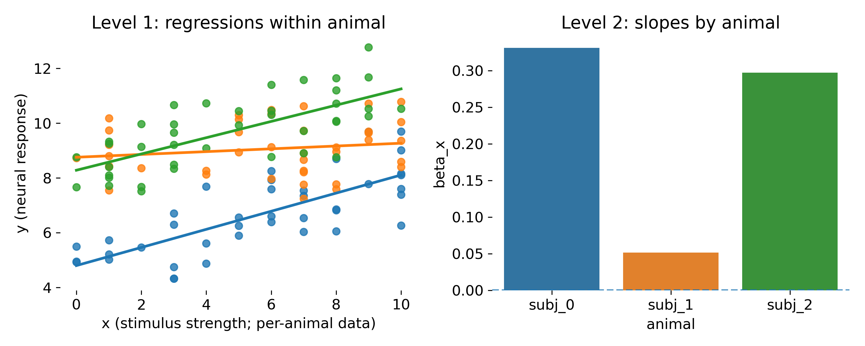 Two stage approach. Left, separate within animal regressions. Right, the estimated slope per animal and the group level mean slope test.
The two stage approach is closer to the hierarchical idea. It estimates a slope per animal, then tests whether the mean slope differs from zero. It can be useful as a simple conceptual bridge to mixed models, but it is statistically inefficient and fragile. It ignores uncertainty in the first stage slopes and it breaks down when per animal sample sizes are small or unbalanced. LMMs unify both stages into a single likelihood, yielding principled uncertainty propagation and shrinkage.
Before we continue, let’s not forget to store the results from the two-stage approach:
rmse, coef, stat, pval = rmse_coef_tstat_pval(lm_level2, "Intercept")
results.loc[len(results)] = ["Two-stage hierarchical (mean slope)", rmse, coef, stat, pval]
LMM random intercept
Finally, we fit a linear mixed model (LMM) with one common slope and random intercepts per animal. This is a standard LMM formulation that captures the idea that animals differ in baseline response, while sharing a common relationship between stimulus strength and response. The random intercepts are modeled as draws from a common Gaussian distribution, allowing for shrinkage toward the population mean.
def plot_lmm_oneslope_randintercept(
    x, y, group, df, model,
    outpath=None, fname="lmm_oneslope_randintercept.png",
    add_text=True):
    """
    LMM: one common slope, random intercept per group.

    Model form: y ~ x + (1 | group)

    Arrows indicate the group-specific random intercept BLUP:
        beta0  ->  beta0 + b0_g

    If add_text=True, annotate the population-level distribution assumption:
        (beta0 + b0_g) ~ N(beta0, Var(b0))
    """

    fig, ax = plt.subplots(figsize=(6.5, 4))
    legend_on = True if df[group].nunique() <= 6 else False
    sns.scatterplot(x=x, y=y, hue=group, data=df, s=35, alpha=0.8, lw=0,
        legend=legend_on,ax=ax)

    palette = itertools.cycle(sns.color_palette())
    x_jitter = -0.2

    base_intercept = float(model.params["Intercept"])
    slope = float(model.params[x])

    # Random-intercept variance estimate (sigma_b^2)
    # For random-intercept-only models, cov_re is 1x1
    try:
        var_b0 = float(model.cov_re.iloc[0, 0])
    except Exception:
        # fallback: sometimes it is exposed as "Group Var" in params
        var_b0 = float(model.params.get("Group Var", np.nan))

    for group_lab, group_df in df.groupby(group):
        x_ = group_df[x].to_numpy()
        color = next(palette)

        re = model.random_effects[group_lab]

        # robustly get intercept BLUP
        if isinstance(re, pd.Series):
            group_offset = float(re.iloc[0])
        elif isinstance(re, dict):
            group_offset = float(list(re.values())[0])
        else:
            group_offset = float(re[0])

        y_pred = base_intercept + slope * x_ + group_offset

        order = np.argsort(x_)
        ax.plot(x_[order], y_pred[order], color=color, linewidth=2.0)

        ax.arrow(
            0 + x_jitter, base_intercept, 0, group_offset,
            head_width=0.25, length_includes_head=True, color=color)

        if add_text and np.isfinite(var_b0) and legend_on:
            ax.text(
                0.15, base_intercept + group_offset,
                f"~N({base_intercept:.3f}, {var_b0:.2f})",
                fontsize=9, color="k", va="center")

        x_jitter += 0.2

    if legend_on:
        ax.legend(frameon=False, bbox_to_anchor=(1.00, 1), loc='upper left')

    # set some proper labels:
    ax.set_xlabel(x + ": stimulus strength")
    ax.set_ylabel(y + ": neural response")

    ax.set_title("LMM: one slope, random intercepts")
    plt.tight_layout()

    if outpath is not None:
        os.makedirs(outpath, exist_ok=True)
        plt.savefig(os.path.join(outpath, fname), dpi=300)
        plt.close()
    else:
        plt.show()
lmm_int = smf.mixedlm("y ~ x", data=df, groups=df["animal"], re_formula="1")
lmm_int_fit = lmm_int.fit(reml=True, method="lbfgs")
print("\nLMM random intercept: y ~ x + (1 | animal)")
print(lmm_int_fit.summary())
LMM random intercept: y ~ x + (1 | animal)
         Mixed Linear Model Regression Results
=======================================================
Model:            MixedLM Dependent Variable: y
No. Observations: 120     Method:             REML
No. Groups:       3       Scale:              1.0275
Min. group size:  40      Log-Likelihood:     -179.6364
Max. group size:  40      Converged:          Yes
Mean group size:  40.0
--------------------------------------------------------
           Coef.  Std.Err.    z    P>|z|  [0.025  0.975]
--------------------------------------------------------
Intercept  7.237     0.977  7.406  0.000   5.322   9.152
x          0.227     0.030  7.596  0.000   0.169   0.286
Group Var  2.760     2.773
=======================================================
This is a typical LMM summary output. It shows the estimated fixed effects (intercept and slope for $x$) along with their standard errors, z statistics, and p values. The estimated slope is 0.227 with a standard error of 0.030, leading to a z statistic of 7.596 and a highly significant p value. Additionally, the variance of the random intercepts (“Group Var”) is estimated to be 2.760.
plot_qq_diagnostics(
    resid=lmm_int_fit.resid.to_numpy(),
    fitted=lmm_int_fit.fittedvalues.to_numpy(),
    groups=df["animal"].to_numpy(),
    title_prefix="LMM random intercept",
    outpath=outpath)

# LMM random intercept plot:
plot_lmm_oneslope_randintercept(x="x", y="y", group="animal", df=df,
                                model=lmm_int_fit,
                                outpath=outpath,
                                add_text=False,
                                fname="LMM_random_intercept_fit.png")

plot_residual_diagnostics(
    residual=lmm_int_fit.resid,
    prediction=lmm_int_fit.fittedvalues,
    group=df["animal"],
    title_prefix="LMM random intercept",
    outpath=outpath,
    fname_prefix="LMM_random_intercept")

rmse, coef, stat, pval = rmse_coef_tstat_pval(lmm_int_fit, "x")
results.loc[len(results)] = ["LMM random intercept", rmse, coef, stat, pval]
Let’s discuss the results. Here is the LMM fit with one common slope and random intercepts per animal:
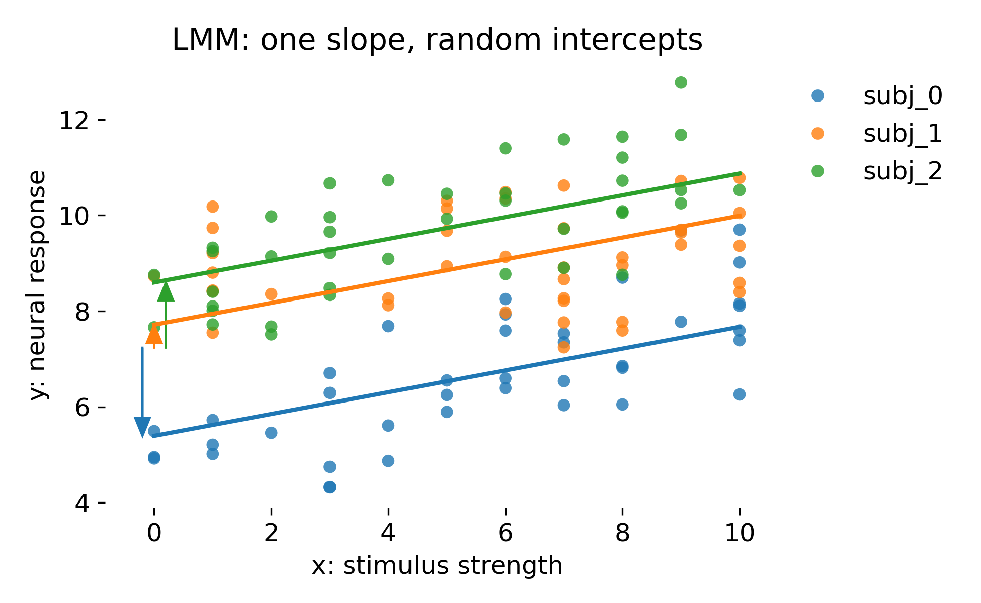 Mixed model with one fixed slope and random intercepts per animal. The colored lines show animal specific fitted lines. Colored arrows indicate the random intercept deviations relative to the population intercept.
This model has the same fixed effect structure as ANCOVA with fixed intercepts, but it treats animal intercepts as random draws from a Gaussian distribution with estimated variance. Conceptually, this is a generative statement about the population. Statistically, it induces partial pooling: Animal intercept estimates are shrunk toward the population intercept depending on how informative each animal’s data are. In balanced data with many observations per animal, fixed intercept ANCOVA and random intercept LMM can look extremely similar in fitted values and residual plots. The main difference is inferential: The LMM yields uncertainty estimates that are consistent with the hierarchical sampling model and supports generalization beyond the observed animals.
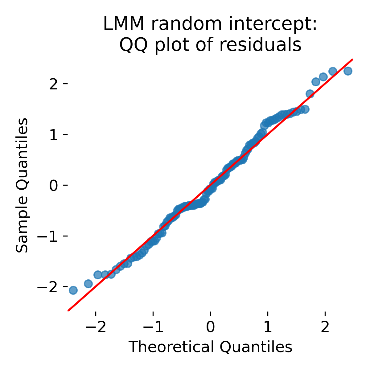
QQ plot of residuals for the random intercept LMM.
Agian, the QQ plot shows approximate normality of residuals under the model. This is similar to the ANCOVA QQ plot. Similarity between ANCOVA and LMM residual plots is expected because both models can capture baseline differences. The crucial point is that model adequacy is not judged solely by residual shapes. Mixed models encode a variance structure and thereby change inference on the fixed effects.
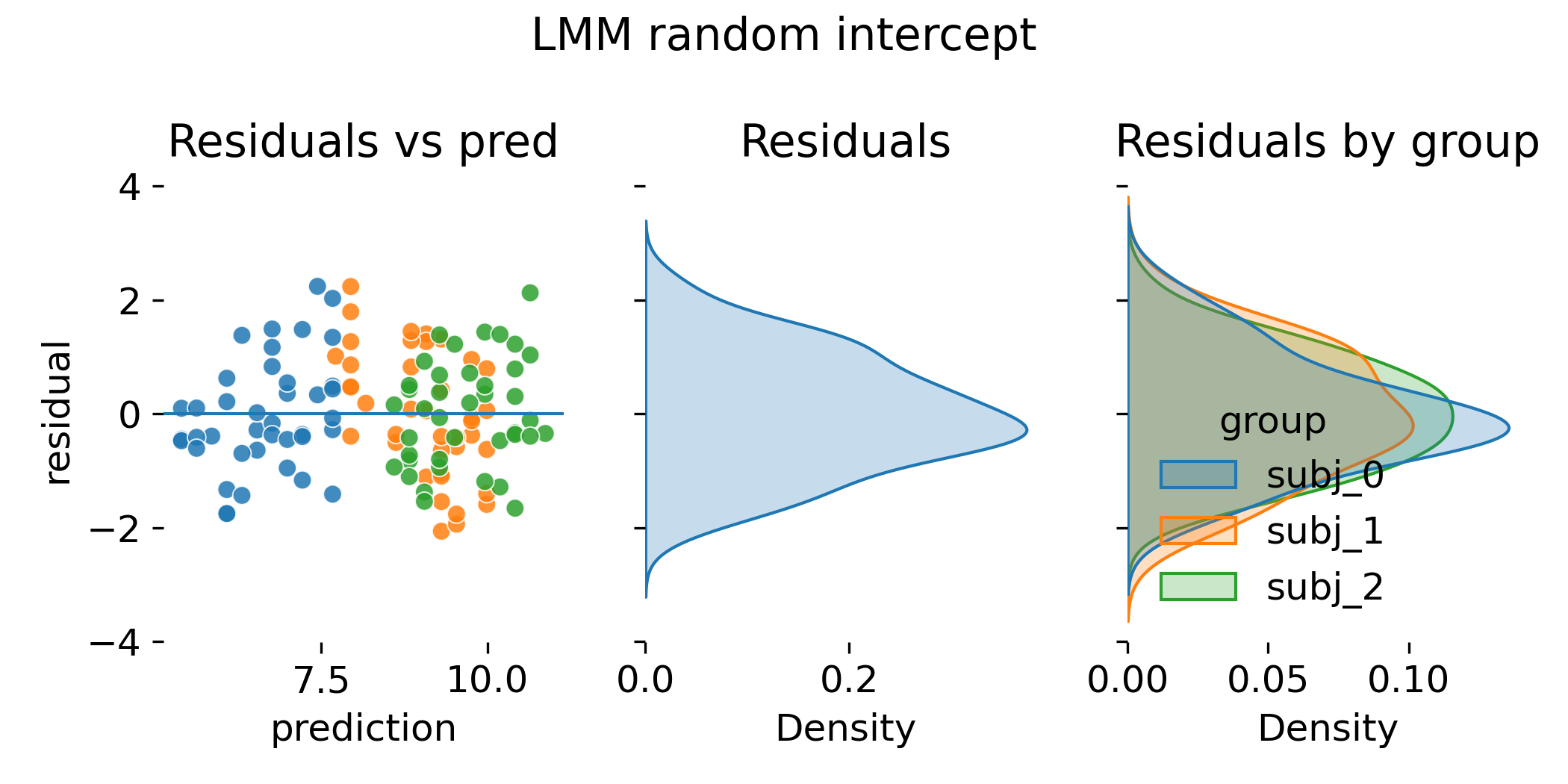 Residual diagnostics for the random intercept LMM.
In this toy dataset, the residual diagnostics plot can look nearly indistinguishable from the ANCOVA fixed intercept diagnostics. That is not a failure. It is a reminder that ANCOVA and LMM can represent similar mean structures in simple balanced settings. The reasons to prefer LMM are more visible when group sizes are small or unbalanced, when there are many groups, and when random slopes matter.
LMM with random intercept and random slope
As a direct follow-up, we fit a more complex LMM that allows both random intercepts and random slopes per animal. This model captures the idea that animals can differ not only in baseline response but also in how strongly their response changes with stimulus strength. The random effects are modeled as draws from a multivariate Gaussian distribution, allowing for covariance between intercepts and slopes.
def plot_lmm_randintercept_randslope(
    x, y, group, df, model,
    outpath=None, fname="lmm_random_intercept_and_slope_fit.png",
    add_arrows=True):
    """
    LMM with random intercept and random slope:
        y ~ x + (1 + x | group)

    Plot:
      * points colored by group
      * dashed black: fixed effects only (population line)
      * solid colored: group-specific lines using BLUPs
    """

    fig, ax = plt.subplots(figsize=(6.5, 4))
    legend_on = True if df[group].nunique() <= 6 else False
    sns.scatterplot(x=x, y=y, hue=group, data=df, s=35, alpha=0.8, lw=0,
                    legend=legend_on,ax=ax)

    xline = np.linspace(df[x].min(), df[x].max(), 200)

    beta0 = float(model.params["Intercept"])
    beta1 = float(model.params[x])

    # population line (fixed effects only)
    ax.plot(xline, beta0 + beta1 * xline, color="k", linestyle="--", linewidth=2.0)

    palette = itertools.cycle(sns.color_palette())
    x_jitter = -0.2

    for group_lab, group_df in df.groupby(group):
        color = next(palette)

        re = model.random_effects[group_lab]
        # For re_formula="1 + x", statsmodels returns two entries (intercept, slope)
        if isinstance(re, pd.Series):
            b0 = float(re.iloc[0])
            b1 = float(re.iloc[1])
        elif isinstance(re, dict):
            vals = list(re.values())
            b0 = float(vals[0])
            b1 = float(vals[1])
        else:
            b0 = float(re[0])
            b1 = float(re[1])

        ax.plot(xline, (beta0 + b0) + (beta1 + b1) * xline, color=color, linewidth=2.5)

        if add_arrows:
            # intercept arrow at x=0
            ax.arrow(
                0 + x_jitter, beta0, 0, b0,
                head_width=0.25, length_includes_head=True, color=color)
            # small slope indication: show delta y over delta x=1 at x=0
            ax.arrow(
                0 + x_jitter, beta0 + b0, 1.0, b1,
                head_width=0.25, length_includes_head=True, color=color)
            x_jitter += 0.2

    ax.set_title("LMM: random intercept and random slope")
    ax.set_xlabel(x + ": stimulus strength")
    ax.set_ylabel(y + ": neural response")

    if legend_on:
        ax.legend(frameon=False, bbox_to_anchor=(1.00, 1), loc='upper left')

    # deactivate left and bottom spines for aesthetics:
    ax.spines['left'].set_visible(False)
    ax.spines['bottom'].set_visible(False)

    plt.tight_layout()
    if outpath is not None:
        os.makedirs(outpath, exist_ok=True)
        plt.savefig(os.path.join(outpath, fname), dpi=300)
        plt.close()
    else:
        plt.show()
lmm_slope = smf.mixedlm("y ~ x", data=df, groups=df["animal"], re_formula="1 + x")
lmm_slope_fit = lmm_slope.fit(reml=True, method="lbfgs")
print("\nLMM random intercept and slope: y ~ x + (1 + x | animal)")
print(lmm_slope_fit.summary())
LMM random intercept and slope: y ~ x + (1 + x | animal)
         Mixed Linear Model Regression Results
=======================================================
Model:            MixedLM Dependent Variable: y
No. Observations: 120     Method:             REML
No. Groups:       3       Scale:              0.8892
Min. group size:  40      Log-Likelihood:     -173.4425
Max. group size:  40      Converged:          Yes
Mean group size:  40.0
-------------------------------------------------------
              Coef.  Std.Err.   z   P>|z| [0.025 0.975]
-------------------------------------------------------
Intercept      7.276    1.246 5.841 0.000  4.834  9.717
x              0.226    0.088 2.570 0.010  0.054  0.398
Group Var      4.564    4.981
Group x x Cov -0.211    0.300
x Var          0.021    0.025
=======================================================
As before, the summary output shows the estimated fixed effects (intercept and slope for $x$) along with their standard errors, z statistics, and p values. The estimated slope is 0.226 with a standard error of 0.088, leading to a z statistic of 2.570 and a significant p value of 0.010. Additionally, the variance of the random intercepts (“Group Var”), the covariance between random intercepts and slopes (“Group x x Cov”), and the variance of the random slopes (“x Var”) are also estimated. What does this tell us? The positive random intercept variance indicates that animals differ in baseline response. The small negative covariance suggests that animals with higher intercepts tend to have slightly lower slopes, although this estimate is uncertain. The positive random slope variance indicates that animals differ in their sensitivity to stimulus strength.
plot_qq_diagnostics(
    resid=lmm_slope_fit.resid.to_numpy(),
    fitted=lmm_slope_fit.fittedvalues.to_numpy(),
    groups=df["animal"].to_numpy(),
    title_prefix="LMM random intercept and\nslope",
    outpath=outpath)

plot_lmm_randintercept_randslope(
    x="x", y="y", group="animal", df=df, model=lmm_slope_fit,
    outpath=outpath, fname="LMM_random_intercept_and_slope_fit.png",
    add_arrows=True)

plot_residual_diagnostics(
    residual=lmm_slope_fit.resid,
    prediction=lmm_slope_fit.fittedvalues,
    group=df["animal"],
    title_prefix="LMM random intercept and slope",
    outpath=outpath,
    fname_prefix="LMM_random_intercept_slope")
# print random effects (BLUPs) per animal:
print("\nRandom effects (BLUPs) from random slope model:")
for k, v in lmm_slope_fit.random_effects.items():
    # v is a Series with entries like "Group" (intercept) and "x"
    print(k, dict(v))
Random effects (BLUPs) from random slope model:
subj_0 {'Group': np.float64(-2.437507828143907), 'x': np.float64(0.10023661532026334)}
subj_1 {'Group': np.float64(1.3737534180704032), 'x': np.float64(-0.15613341169987927)}
subj_2 {'Group': np.float64(1.063754410072425), 'x': np.float64(0.055896796379645015)}
We additionally print the random effects (BLUPs) per animal. Each animal has a random intercept (“Group”) and a random slope (“x”). For example, subj_0 has a random intercept of approximately -2.44 and a random slope of approximately 0.10. These values indicate how much the animal’s intercept and slope deviate from the population values.
Let’s now discuss the diagnotics plots. Here is the LMM fit with random intercepts and random slopes per animal:
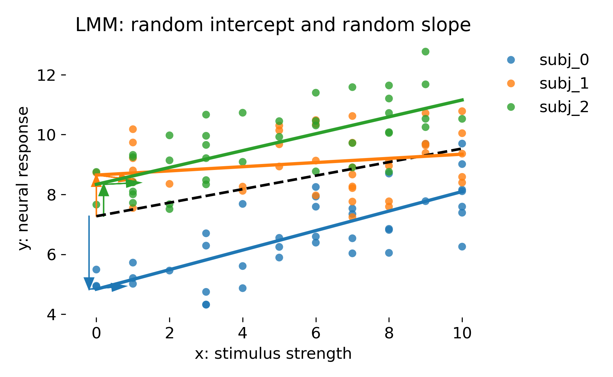 Mixed model with random intercepts and random slopes per animal. The dashed black line is the population line (fixed effects only). Colored lines are animal specific fits using random effect BLUPs.
This model reflects a very common situation in neuroscience: Not only baselines differ between animals, but stimulus sensitivity differs as well. The dashed line represents $\beta_0 + \beta_1 x$. Each animal has its own intercept shift $b_{0i}$ and slope shift $b_{1i}$, producing a family of lines. The vertical colored arrows indicate intercept deviations from the population line at $x=0$. The additional horizontal colored arrows indicate slope deviations in the following sense: The arrow is drawn with $\Delta x = 1$ and vertical component $\Delta y = b_{1i}$. It visualizes how much steeper or flatter the animal’s line is compared to the population line, evaluated locally at the intercept. These arrows are a representation of the random slope term and should not be interpreted as separate parameters. They are graphical cues for $b_{0i}$ and $b_{1i}$.
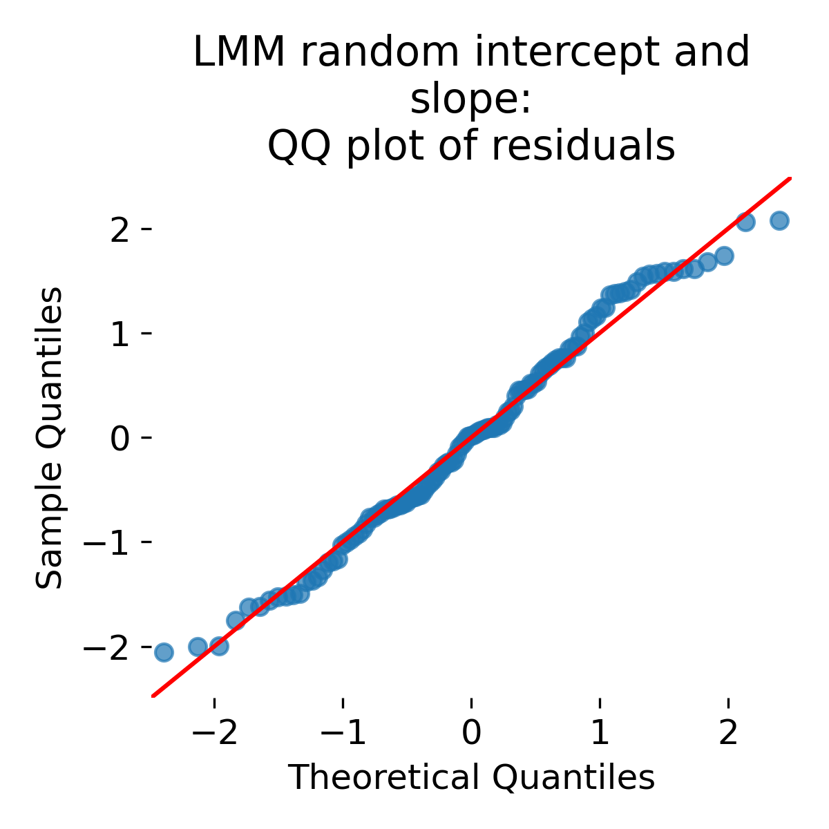
QQ plot of residuals for the random intercept and slope LMM.
Depending on the simulation and the number of animals, residual distributions can broaden or narrow compared to simpler models. A narrower residual distribution does not automatically imply a better model. In mixed models, part of what looks like “tight residuals” can come from overfitting group specific parameters when groups are treated as fixed and numerous. Mixed models instead allocate variance to random effect components, which is often the correct representation of how data were generated. Diagnostics should be read in conjunction with the model’s intended generalization target.
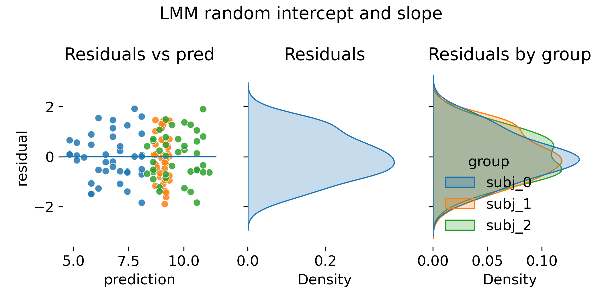 Residual diagnostics for the random intercept and slope LMM.
In all previous models, we have seen that residual diagnostics can look similar between ANCOVA and LMM, and so it is here. This is because both allow group specific slopes. The decisive difference is not the existence of group specific slopes but how they are estimated and regularized. LMMs shrink group slopes toward the population slope when group specific evidence is weak. This matters dramatically when groups are many and per group data are scarce.
We will make this clear by another type of comparison, for which we will implement a last model: ANCOVA with interaction.
Before that, let’s not forget to store the results from the random intercept and slope LMM:
rmse, coef, stat, pval = rmse_coef_tstat_pval(lmm_slope_fit, "x")
results.loc[len(results)] = ["LMM random intercept + slope", rmse, coef, stat, pval]
ANCOVA full model with interaction
To complete the comparison, we fit an ANCOVA model with interaction between stimulus strength and animal. This model allows each animal to have its own intercept and slope, estimated as fixed parameters without pooling. This is the direct fixed effects analogue to the random intercept and slope LMM.
def plot_ancova_fullmodel(x, y, group, df, model, outpath=None, fname="ANCOVA_fullmodel.png"):
    """
    ANCOVA full model with interaction:
      y ~ x * C(group)
    Equivalent to:
      y ~ x + C(group) + x:C(group)

    Plot:
      * points per group
      * dashed black lines: "no-interaction" reference with group intercept offsets
            y_ref_g(x) = Intercept + beta_x * x + offset_g
        where beta_x is the slope of the reference group (from the fitted interaction model)
        and offset_g is the group intercept shift (C(group)[T.g]).
      * colored lines: full interaction model predictions within each group
      * arrows: show offset_g at x=0
    """
    legend_on = True if df[group].nunique() <= 6 else False
    g = sns.lmplot(x=x, y=y, hue=group, data=df, fit_reg=False, height=4, aspect=1.6,
                   legend=False)
    ax = g.ax

    palette = itertools.cycle(sns.color_palette())
    x_jitter = -0.2

    base_intercept = float(model.params["Intercept"])
    base_slope = float(model.params[x])  # slope for the reference group in the interaction model

    for group_lab, group_df in df.groupby(group):
        color = next(palette)

        x_ = group_df[x].to_numpy()
        order = np.argsort(x_)
        x_sorted = x_[order]

        # --- fixed intercept offset for this group (reference group has 0) ---
        key = f"C({group})[T.{group_lab}]"
        group_offset = float(model.params[key]) if key in model.params else 0.0

        # --- dashed reference: same slope, different intercepts (NO interaction slopes) ---
        y_ref = base_intercept + base_slope * x_sorted + group_offset
        ax.plot(x_sorted, y_ref, color="k", linestyle="--", linewidth=2.0, zorder=5)

        # --- colored: full interaction predictions (group specific slope + intercept) ---
        y_pred = np.asarray(model.predict(group_df))[order]
        ax.plot(x_sorted, y_pred, color=color, linewidth=2.5)

        # --- arrow indicates the intercept shift at x=0 ---
        ax.arrow(0 + x_jitter, base_intercept, 0, group_offset,
                 head_width=0.25, length_includes_head=True, color=color)
        x_jitter += 0.2

    # deactivate left and bottom spines for aesthetics:
    ax.spines['left'].set_visible(False)
    ax.spines['bottom'].set_visible(False)

    # set proper x and y labels:
    ax.set_xlabel(x + ": stimulus strength")
    ax.set_ylabel(y + ": neural response")

    # if legend_on, put the legend right outside the plot
    if legend_on:
        ax.legend(frameon=False, bbox_to_anchor=(1.00, 1), loc='upper left')

    ax.set_title("ANCOVA full: group specific intercepts\nand slopes(interaction)")
    plt.tight_layout()

    if outpath is not None:
        os.makedirs(outpath, exist_ok=True)
        plt.savefig(os.path.join(outpath, fname), dpi=300)
        plt.close()
    else:
        plt.show()
ancova_full = smf.ols("y ~ x * C(animal)", data=df).fit()
print("\nANCOVA full: y ~ x * C(animal)")
print(ancova_full.summary().tables[1])
ANCOVA full: y ~ x * C(animal)
=========================================================================================
                            coef    std err          t      P>|t|      [0.025      0.975]
-----------------------------------------------------------------------------------------
Intercept                 4.7980      0.303     15.821      0.000       4.197       5.399
C(animal)[T.subj_1]       3.9579      0.442      8.956      0.000       3.082       4.833
C(animal)[T.subj_2]       3.4834      0.411      8.480      0.000       2.670       4.297
x                         0.3309      0.047      7.048      0.000       0.238       0.424
x:C(animal)[T.subj_1]    -0.2796      0.067     -4.144      0.000      -0.413      -0.146
x:C(animal)[T.subj_2]    -0.0337      0.068     -0.495      0.622      -0.169       0.101
=========================================================================================
From the summary output, we see the estimated coefficients for the intercept, the animal-specific intercept offsets, the slope for $x$, and the interaction terms representing animal-specific slope adjustments. Each animal has its own intercept and slope, estimated as fixed effects. Interpreting the coeffiecients, we find that the reference animal (subj_0) has an intercept of 4.7980 and a slope of 0.3309. Animal subj_1 has an intercept offset of 3.9579 and a slope adjustment of -0.2796, resulting in an effective intercept of 8.7559 and a slope of 0.0513. Animal subj_2 has an intercept offset of 3.4834 and a slope adjustment of -0.0337, leading to an effective intercept of 8.2814 and a slope of 0.2972. What does this indicate? It means that animal subj_1 has a much flatter response to stimulus strength compared to the reference animal, while animal subj_2 has a slope closer to the reference but still slightly reduced.
plot_ancova_fullmodel(
    x="x", y="y", group="animal", df=df, model=ancova_full,
    outpath=outpath, fname="ANCOVA_full_interaction.png")

plot_residual_diagnostics(
    residual=ancova_full.resid,
    prediction=ancova_full.predict(df),
    group=df["animal"],
    title_prefix="ANCOVA full (interaction)",
    outpath=outpath,
    fname_prefix="ANCOVA_full")

rmse, coef, stat, pval = rmse_coef_tstat_pval(ancova_full, "x")
results.loc[len(results)] = ["ANCOVA full (interaction)", rmse, coef, stat, pval]
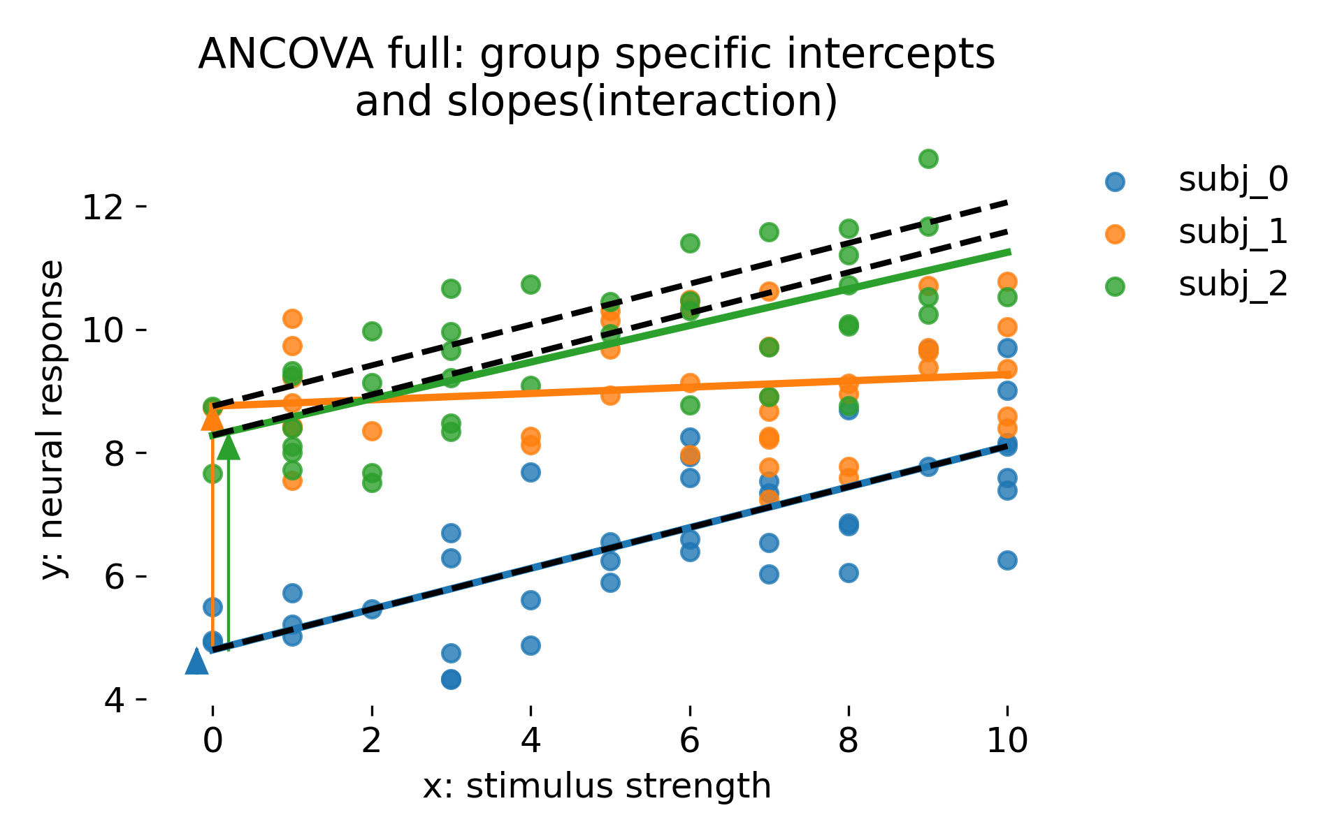 ANCOVA with group specific intercepts and group specific slopes via interaction terms. Dashed black lines show a no interaction reference in which groups differ only by intercept offsets but share the reference slope. Colored lines are full interaction fits. Arrows indicate intercept offsets.
This model assigns each group its own slope and intercept as fixed parameters. With few groups and many observations per group, this can be perfectly reasonable. However, it does not encode any population distribution over slopes and intercepts. Each group parameter is estimated independently, and the model therefore lacks shrinkage. This tends to exaggerate differences between groups when groups are numerous or poorly sampled. It also makes generalization beyond the observed groups conceptually unclear because the model treats group identities as fixed categories rather than as random draws.
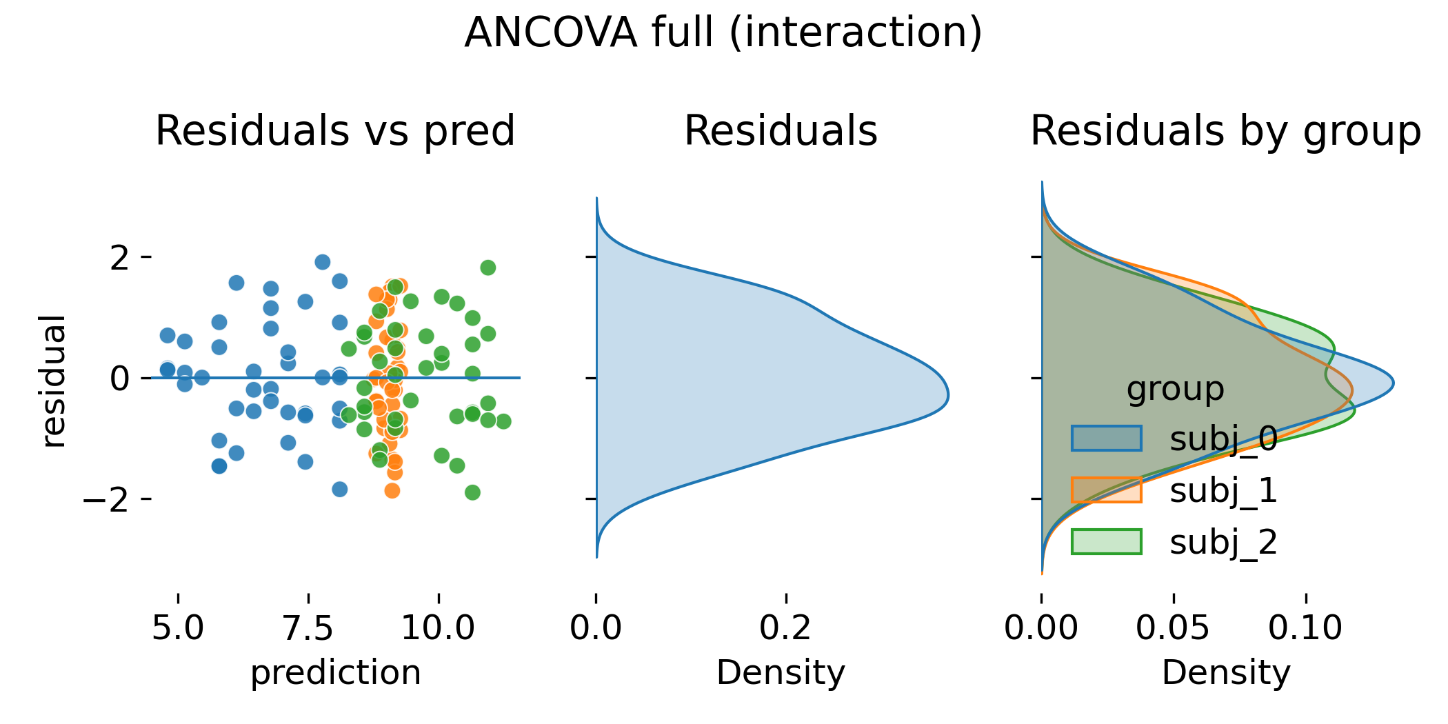 Residual diagnostics for ANCOVA with interaction.
Again, residual plots can look similar to the random slope LMM. A slightly narrower residual distribution in ANCOVA does not imply superiority. With many groups, an interaction model can soak up variance by fitting a large number of slope parameters. That may improve in sample fit but it increases variance of group specific estimates and can harm generalization. Mixed models trade a small amount of in sample fit for stability by regularizing group effects through a variance component.
Shrinkage: Why LMM and ANCOVA can look similar yet behave differently
Residual plots do not show shrinkage directly. Shrinkage is a property of the conditional group estimates. A direct visualization is to compare group specific slopes estimated by ANCOVA interaction to the group specific slopes implied by the LMM BLUPs:
def extract_group_slopes_from_ancova_full(model, df, group_col="animal", x_col="x"):
    """
    For y ~ x * C(group), compute the slope per group:
      slope_group = beta_x + beta_{x:C(group)[T.group]}
    Reference group gets just beta_x.
    """
    beta_x = float(model.params[x_col])
    slopes = {}
    groups = df[group_col].unique()
    for g in groups:
        key = f"{x_col}:C({group_col})[T.{g}]"
        slopes[g] = beta_x + (float(model.params[key]) if key in model.params else 0.0)
    return slopes

def extract_group_slopes_from_lmm(model, df, group_col="animal", x_col="x"):
    """
    For MixedLM with re_formula="1 + x", slope per group is:
      slope_group = beta_x + b1_group
    """
    beta_x = float(model.params[x_col])
    slopes = {}
    for g in df[group_col].unique():
        re = model.random_effects[g]
        if isinstance(re, pd.Series):
            b1 = float(re.iloc[1])
        else:
            b1 = float(re[1])
        slopes[g] = beta_x + b1
    return slopes

def plot_slope_comparison(slopes_ancova, slopes_lmm, outpath, fname="slope_comparison.png"):
    keys = sorted(set(slopes_ancova.keys()) & set(slopes_lmm.keys()))
    y1 = np.array([slopes_ancova[k] for k in keys])
    y2 = np.array([slopes_lmm[k] for k in keys])

    plt.figure(figsize=(6, 5))
    for subject_i, subject in enumerate(keys):
        plt.scatter(y1[subject_i], y2[subject_i], s=40, alpha=0.8)
    lo = min(y1.min(), y2.min())
    hi = max(y1.max(), y2.max())
    plt.plot([lo, hi], [lo, hi], linewidth=2.0)
    plt.xlabel("Group slope, ANCOVA full")
    plt.ylabel("Group slope, LMM BLUP")
    plt.title("Group-specific slopes\nANCOVA full versus LMM (shrinkage)")
    plt.tight_layout()
    plt.savefig(os.path.join(outpath, fname), dpi=300)
    plt.close()
slopes_ancova = extract_group_slopes_from_ancova_full(ancova_full, df, group_col="animal", x_col="x")
slopes_lmm = extract_group_slopes_from_lmm(lmm_slope_fit, df, group_col="animal", x_col="x")
plot_slope_comparison(slopes_ancova, slopes_lmm, outpath=outpath)
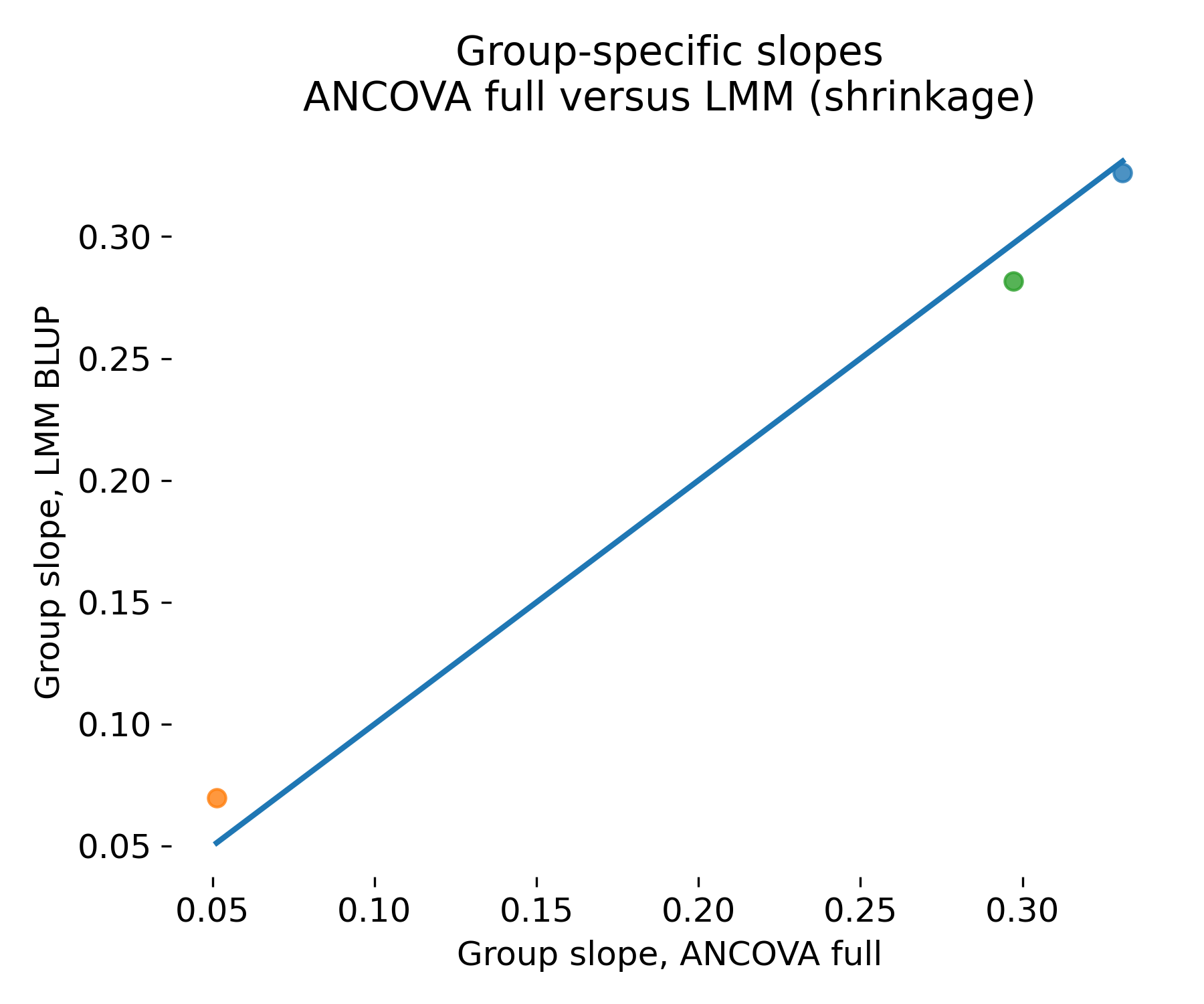 Group specific slope comparison between ANCOVA full and LMM. The horizontal axis shows group slope estimates from the ANCOVA interaction model. The vertical axis shows group slope estimates from the LMM via BLUPs. The diagonal indicates equality.
In this particular toy dataset, the three animals fall essentially on the diagonal, so the plot does not show a dramatic separation between ANCOVA and LMM. This is expected given how the dataset was generated and how much information each animal carries: There are only three animals, each with many observations, and the design is balanced. In that regime, the group specific slopes are well identified from each animal’s own data, so the mixed model has little reason to shrink them strongly toward the population slope. In other words, the conditional estimates under the LMM end up close to the corresponding group specific estimates one would obtain from a fixed interaction model. The visual message here is therefore not “shrinkage is large”, but rather “shrinkage can be negligible when each group is well sampled”.
This does not weaken the conceptual distinction. The distinction is that ANCOVA with interactions treats each group’s slope as an independent fixed parameter, while the LMM treats slopes as random draws from a population distribution with an estimated variance. The mixed model therefore induces partial pooling: The group specific slope estimate is pulled toward the population slope by an amount that depends on how informative that group is relative to the estimated between group variance and the residual noise level. If a group has little information, for example few trials, high noise, or limited spread in the predictor $x$, the LMM shrinks its slope toward the population value. If a group has a lot of information, shrinkage becomes small and the group estimate approaches what a group specific fit would deliver.
The practical consequence is that ANCOVA and LMM can look nearly identical in residual plots and even in fitted lines in small, balanced, high information examples, yet they behave differently once the realistic regime is entered: many animals, few observations per animal, unbalanced sampling, or correlated random intercept and slope structure. In those regimes, ANCOVA interaction slopes can fluctuate widely because each slope is estimated without regularization, while LMM slopes remain stable because the model borrows strength across animals through the random effects variance structure. This is the setting in which shrinkage becomes visually obvious and methodologically decisive.
Results summary table
Throughout the model fitting, we have collected RMSE, estimated $x$ coefficient, its test statistic, and p value for each model:
print(results)
| Model | RMSE | Coef_x | Stat_x | Pval_x |
|---|---|---|---|---|
| OLS global (biased SE) | 1.698294 | 0.189848 | 3.831865 | 2.053972e-04 |
| ANCOVA fixed intercepts | 1.013649 | 0.227828 | 7.607805 | 8.031926e-12 |
| Two-stage hierarchical (mean slope) | 0.152641 | 0.226438 | 2.569429 | 1.239321e-01 |
| LMM random intercept | 1.005103 | 0.227469 | 7.596175 | 3.050128e-14 |
| LMM random intercept + slope | 0.927902 | 0.225858 | 2.570196 | 1.016411e-02 |
| ANCOVA full (interaction) | 0.942923 | 0.330894 | 7.048024 | 1.478715e-10 |
Two clarifications are important before interpreting the numbers. First, RMSE is an in-sample fit measure and not the goal of inferential modeling. Lower RMSE can be achieved simply by adding parameters and does not by itself imply a better inferential model. Second, test statistics are not strictly comparable across models: OLS-based models report t statistics, whereas statsmodels reports Wald z statistics for mixed models.
With this in mind, several clear patterns emerge from the table.
The global OLS model performs worst. Its RMSE is highest, and the slope estimate is attenuated. This reflects a misspecification: Repeated measurements within animals are treated as independent, inflating residual variance and biasing standard errors.
Introducing animal-specific intercepts via ANCOVA substantially improves the fit and stabilizes the slope estimate. The corresponding LMM with random intercepts yields nearly identical fixed-effect estimates and RMSE in this balanced toy dataset. This similarity is expected. However, the interpretation differs: ANCOVA conditions on the observed animals, while the LMM treats animals as a random sample from a population and explicitly estimates between-animal variance.
The two-stage hierarchical approach illustrates a common pitfall. By collapsing each animal to a single slope estimate, the effective sample size for inference becomes the number of animals. As a result, statistical power is low, and uncertainty is underestimated in an ad hoc way. This approach discards information that mixed models retain naturally.
Allowing random slopes in the LMM changes the inferential question. The fixed effect now represents the population-average slope in the presence of genuine between-animal variability. Consequently, uncertainty increases compared to the random-intercept-only model, even though RMSE decreases slightly. This is not a weakness but a more honest representation of heterogeneity.
Finally, the full ANCOVA interaction model assigns a separate fixed slope to each animal. While its RMSE is comparable to the random-slope LMM, it lacks any pooling across animals. As a result, group-specific slopes can become unstable when data are sparse. The mixed model addresses this through shrinkage, yielding more conservative and robust group-level estimates.
Overall, the table shows that models can appear similar in terms of residuals or RMSE, yet differ fundamentally in how they represent population structure, uncertainty, and generalizability. This distinction is central when choosing between ANCOVA-style models and linear mixed models.
A simulator designed to highlight where LMMs dominate ANCOVA
To make the difference between ANCOVA and LMM both visually and methodologically obvious, we now simulate data in a regime that is common in practice and challenging for fixed effects approaches. We use many animals, few observations per animal, an unbalanced design, correlated random intercepts and slopes, and group shifted $x$ distributions. This setting is problematic for ANCOVA interaction because it estimates a separate slope for each animal with little data support. The LMM, in contrast, pools information across animals through the random effect covariance structure and thereby yields stable group estimates.
Let’s write a new simulator for this scenario:
def simulate_animal_data_lmm_friendly(
    seed=0,
    n_animals=40,
    n_obs_min=3,
    n_obs_max=8,
    beta0=8.0,
    beta1=0.25,
    sigma_animal_intercept=2.5,
    sigma_animal_slope=0.35,
    rho_intercept_slope=-0.6,
    sigma_noise=1.0,
    x_mode="group_shifted"):
    """
    LMM-friendly simulation.

    Key features:
    * many groups, few observations per group (and unbalanced)
    * random intercepts AND random slopes
    * correlated random effects (b0,b1)
    * optional group-shifted x distributions

    x_mode:
      "shared"        -> all groups draw x from the same distribution
      "group_shifted" -> each group sees its own x-range, causing confounding risk
    """
    rng = np.random.default_rng(seed)
    animals = [f"subj_{i}" for i in range(n_animals)]

    # correlated random effects (b0,b1) per animal
    cov = np.array([
        [sigma_animal_intercept**2, rho_intercept_slope*sigma_animal_intercept*sigma_animal_slope],
        [rho_intercept_slope*sigma_animal_intercept*sigma_animal_slope, sigma_animal_slope**2]
    ])
    b = rng.multivariate_normal(mean=[0.0, 0.0], cov=cov, size=n_animals)
    b0 = b[:, 0]
    b1 = b[:, 1]

    rows = []
    for i, a in enumerate(animals):
        n_obs = int(rng.integers(n_obs_min, n_obs_max + 1))

        if x_mode == "shared":
            x = rng.integers(0, 11, size=n_obs).astype(float)
        else:
            # each animal sees a shifted x-window
            center = float(rng.integers(0, 11))
            x = center + rng.normal(0.0, 1.0, size=n_obs)
            x = np.clip(x, 0.0, 10.0)

        mu = (beta0 + b0[i]) + (beta1 + b1[i]) * x
        y = mu + rng.normal(0.0, sigma_noise, size=n_obs)

        for xx, yy in zip(x, y):
            rows.append({"animal": a, "x": float(xx), "y": float(yy)})

    return pd.DataFrame(rows)
and create a dataset with 40 animals, 3 to 8 observations per animal (=unbalanced), correlated random effects, and group shifted $x$ distributions:
df = simulate_animal_data_lmm_friendly(
        seed=41,
        n_animals=40,
        n_obs_min=3,
        n_obs_max=8,
        beta0=8.0,
        beta1=0.25,
        sigma_animal_intercept=2.5,
        sigma_animal_slope=0.35,
        rho_intercept_slope=-0.6,
        sigma_noise=1.0,
        x_mode="group_shifted")
Here is how the data looks (again color-coded by animal):
 Raw data by animal (color-coded) in an LMM friendly regime with many groups and few observations per group. Each animal has its own x-range, causing potential confounding between animal effects and stimulus strength.
In this run, we do not repeat all plots for the sake of brevity. Instead, we focus on the key differences that emerge in this more challenging regime. The key plot is again the slope comparison between ANCOVA interaction and LMM random slopes, which we have introduced as the last step above:
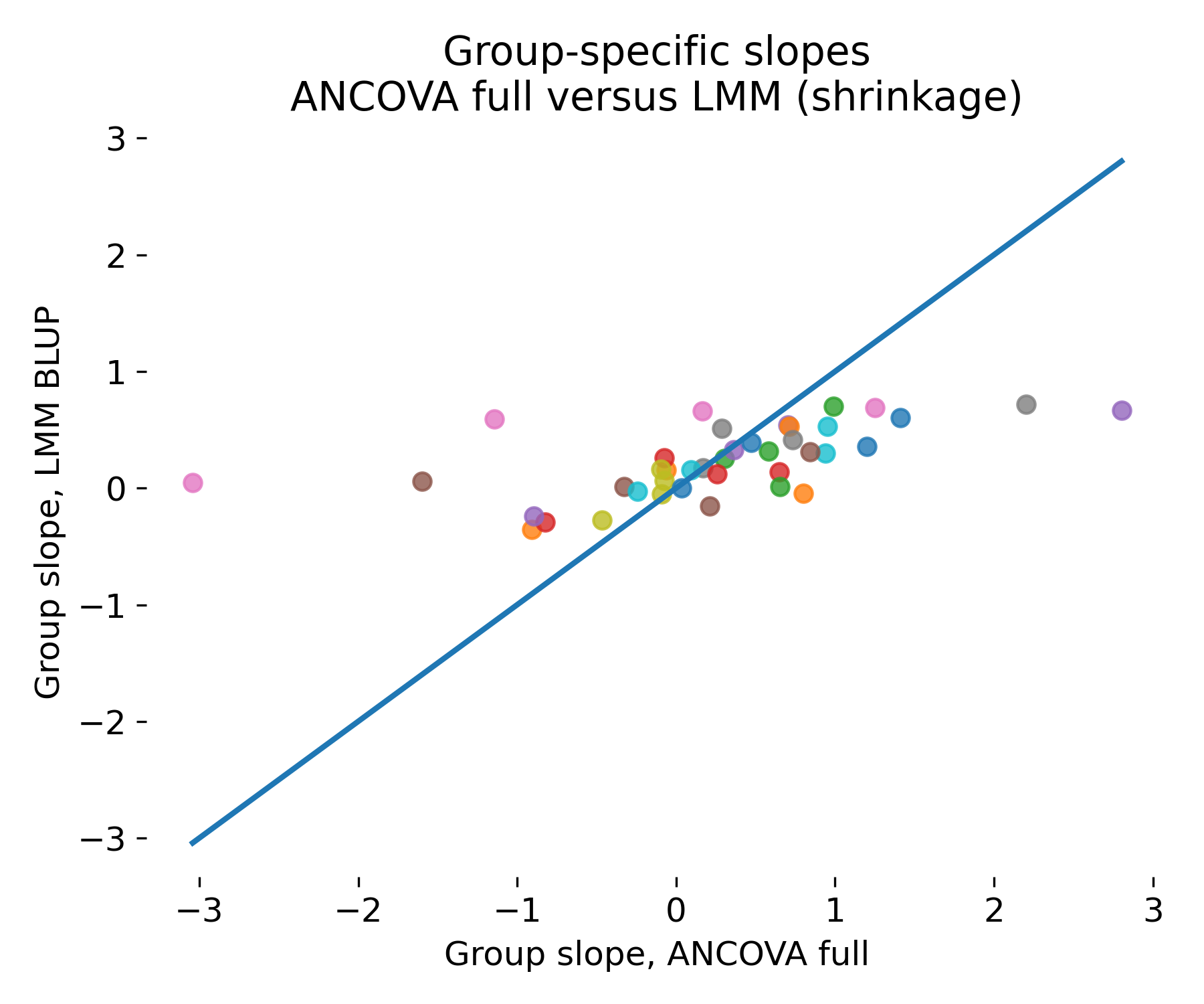 Group specific slope comparison in an LMM friendly regime with many groups and few observations per group. ANCOVA interaction slope estimates scatter widely, while LMM BLUP slopes are pulled toward the population mean.
Here we see, that the ANCOVA interaction model exhibits high variance because it assigns one slope parameter per group without regularization. With few observations per group, these slope estimates fluctuate substantially due to noise. The LMM explicitly models that slopes are drawn from a population distribution and therefore shrinks noisy slopes. This stabilizes group specific estimates, improves out of sample behavior, and yields an interpretable variance component for slope heterogeneity. In unbalanced designs, this advantage becomes larger because groups with fewer points are automatically pooled more strongly, which matches what one would do by hand if forced. The constellation of many groups with few observations per group is, thus, exactly the regime where mixed models are not merely aesthetically preferable but methodologically necessary.
This qualitative difference is also reflected quantitatively when we compare the model summaries obtained for this dataset. As before, we collected RMSE, the estimated population-level slope, and its associated test statistic for each model:
| Model | RMSE | Coef_x | Stat_x | Pval_x |
|---|---|---|---|---|
| OLS global (biased SE) | 2.196989 | 0.109376 | 2.280728 | 0.023513 |
| ANCOVA fixed intercepts | 1.087251 | 0.274975 | 3.200333 | 0.001618 |
| Two-stage hierarchical (mean slope) | 0.993636 | 0.246683 | 1.570156 | 0.124458 |
| LMM random intercept | 0.993749 | 0.228003 | 3.337680 | 0.000845 |
| LMM random intercept + slope | 0.913017 | 0.233452 | 2.536810 | 0.011187 |
| ANCOVA full (interaction) | 1.022376 | 1.412284 | 2.285398 | 0.023740 |
Compared to the balanced toy dataset, the differences between model classes now become much more pronounced.
The global OLS model again performs poorly. Treating all observations as independent leads to an attenuated slope estimate and inflated residual variance. This behavior is consistent across both simulations and reflects a fundamental misspecification when repeated measures are present.
ANCOVA with fixed intercepts improves over global OLS, but its slope estimate shifts noticeably and its RMSE remains relatively high. In this regime, fixed intercept ANCOVA begins to absorb structure that actually belongs to slope heterogeneity, because differences between animals are no longer limited to baseline offsets.
The two-stage hierarchical approach deteriorates further. With many animals and only a handful of observations per animal, collapsing each animal to a single slope leaves too little information for reliable inference. The resulting estimate is noisy and statistically inconclusive, highlighting why this approach is generally discouraged outside of very simple settings.
The contrast between ANCOVA interaction and LMM with random slopes is now stark. The ANCOVA interaction model produces an higher slope estimate for the reference group. This is not a subtle effect: Assigning one fixed slope per animal without pooling leads to unstable estimates when data per group are sparse and $x$ ranges differ across animals. The inflated coefficient, while not beeing extremely large, in the table is a direct numerical manifestation, of this instability.
In contrast, the mixed model with random slopes remains well behaved. Its population-level slope stays close to the generative value (0.25), and its uncertainty reflects genuine between-animal variability rather than overfitting noise. This is important to note so that we do not misinterpret the higher variance in the LMM slope estimate as a weakness compared, e.g., to the two-stage approach or OLS models. The higher uncertainty is a more honest representation of the inferential question being asked: What is the average slope in a population with heterogeneous slopes? The mixed model answers this question correctly, while the two-stage approach lacks power and OLS/ANCOVA misrepresent uncertainty due to ignored dependencies. And the modest reduction in RMSE relative to the random-intercept model is secondary; the crucial point is that the meaning of the fixed effect remains stable across datasets with very different structures.
Taken together, the comparison of both result tables reinforces the central message of our little study. In balanced designs, ANCOVA and LMMs can yield superficially similar results. Once the data regime shifts to many groups, few observations per group, unbalanced sampling, and heterogeneous covariate ranges, fixed-effects approaches break down in characteristic ways. Linear mixed models do not merely fit better; they encode the correct statistical assumptions about how group-level effects arise and therefore remain interpretable and robust where ANCOVA does not.
Summary (incl. decision table)
So, what do we gain from this exercise? When should we use ANCOVA, and when are linear mixed models the better choice?
The message is not that ANCOVA is fundamentally wrong or obsolete. In simple, balanced designs with a small number of groups and many observations per group, ANCOVA models can describe the data well and can be entirely appropriate, provided that inference is explicitly restricted to the observed groups.
The central distinction lies elsewhere. ANCOVA treats group effects as fixed and conditional on the specific groups in the dataset. Linear mixed models, in contrast, treat groups as a random sample from a population and explicitly model the resulting variance structure. This difference becomes crucial as soon as experiments move beyond small, balanced designs.
In practice, LMMs become the natural modeling choice when any of the following apply:
- groups are sampled from a population,
- group sizes are unbalanced,
- the number of groups is large, or
- group-specific effects must be estimated robustly under limited data.
In these settings, fixed-effects approaches either break down or answer a different inferential question than intended.
In the table below, I tried to summarize our findings and provide guidance on when to use which model type. It is not a formal proof, but it reflects practical experience and the simulations we have seen:
| Data structure and goal | OLS or t test | ANOVA or ANCOVA fixed intercept | ANCOVA with interaction (fixed slopes per group) | LMM random intercept | LMM random intercept + slope |
|---|---|---|---|---|---|
| Truly independent observations | ✅ | ✅ | ✅ | ✅ | ✅ |
| Repeated measures within subject or animal | ❌ | sometimes | rarely | ✅ | ✅ |
| Few groups, many observations per group, interest only in these groups | sometimes | ✅ | ✅ | ✅ | ✅ |
| Many groups, few observations per group | ❌ | ❌ | ❌ | ✅ | ✅ |
| Unbalanced group sizes | ❌ | sometimes | unstable | ✅ | ✅ |
| Group specific baselines only | ❌ | ✅ | ✅ | ✅ | ✅ |
| Group specific slopes, but groups are sampled from a population | ❌ | ❌ | conceptually awkward | sometimes | ✅ |
| Correlated random intercept and slope structure | ❌ | ❌ | ❌ | partial | ✅ |
| Need stable group estimates and generalization beyond observed groups | ❌ | limited | ❌ | ✅ | ✅ |
The two core strengths of linear mixed models are variance structure modeling and shrinkage. Modeling the variance structure ensures that uncertainty in fixed effects correctly reflects dependence induced by grouping. Shrinkage stabilizes group-specific estimates by borrowing strength across groups, especially when per-group data are sparse.
These properties are not cosmetic. They directly address the realities of real world data, especially in neuroscience, where repeated measurements, nested designs, unequal sampling, and heterogeneous responses are the norm rather than the exception.
Outlook: Generalized linear mixed models (GLMMs)
Linear mixed models assume Gaussian residuals and a linear mean structure. In many applications this is a reasonable approximation, but in others it is not. Binary outcomes, counts, proportions, and bounded response variables violate the Gaussian assumption and therefore require a different observation model. In such cases, the appropriate extension is a generalized linear mixed model (GLMM).
A GLMM combines the hierarchical structure of LMMs with the flexible likelihood framework of generalized linear models. The linear predictor is linked to the expected value of the response through a link function $g(\cdot) $, while the mixed effect structure is preserved. In this sense, GLMMs are not an alternative to LMMs, but their natural generalization to non Gaussian data.
A canonical formulation is
\[\begin{align} g(\mathbb{E}[y_{ij}]) &= \mathbf{x}_{ij}^\top \boldsymbol{\beta} + \mathbf{z}_{ij}^\top \mathbf{b}_i, \end{align}\]where $g$ is a link function such as the logit for binary responses or the log for count data. The fixed effects $\boldsymbol{\beta} $ and random effects $\mathbf{b}_i$ have the same interpretation as in LMMs. What changes is the observation model: The residuals are no longer Gaussian, and the likelihood is defined by the chosen distribution, for example Bernoulli or Poisson.
Inference in GLMMs is more involved because closed form solutions are generally unavailable. Estimation therefore relies on approximations or sampling based methods. Nevertheless, the conceptual hierarchy remains identical to that of LMMs, and the same principles regarding grouping, variance components, and shrinkage apply.
In Python, support for GLMMs is available through several libraries. statsmodels provides limited frequentist functionality, while PyMC and Bambi offer Bayesian GLMMs with flexible model specification and formula based interfaces.
As with linear mixed models, careful model diagnostics are essential. Convergence must be checked, fitted values and residual like quantities should be inspected, and the choice of distribution and link function should be guided by the data generating process and the scientific question rather than by convenience.
Conclusion
Linear mixed models are a powerful tool for analyzing hierarchical and grouped data, not only in neuroscience. They provide a principled way to account for dependencies, model variance structures, and stabilize group specific estimates through shrinkage. Compared to traditional ANCOVA approaches, LMMs offer greater flexibility and interpretability, especially in complex experimental designs with many groups and unbalanced data. By understanding when and how to apply LMMs, you can indeed improve the validity and generalizability of your statistical inferences and better capture the underlying (biological) processes.
You can find the complete code for the simulations and analyses presented in this post in this GitHub repositoryꜛ.
References
- Edouard Duchesnayꜛ’s tutorial LMM tutorialꜛ from his online course on Statistical Learning in Pythonꜛ
- Andrew Gelman and Jennifer Hill, Data analysis using regression and multilevel hierarchical models, 2006, Cambridge University Press, ISBN: 978-0521686891
- Brady T. West, Kathleen B. Welch, Andrzej T. Galecki, Linear Mixed Models: A Practical Guide Using Statistical Software, 2014, 2nd edition, ISBN: 978-1032019321, online available hereꜛ
- Andrzej Gałecki, Tomasz Burzykowski, Linear Mixed-Effects Models Using R: A Step-by-Step Approach, 2015, Springer, ISBN: 978-1489996671


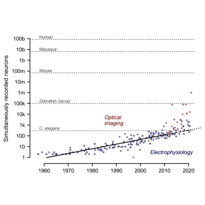


comments