Manual Ca²⁺ signal extraction with Fiji and a spreadsheet tool

This is a step-by-step tutorial on extracting Ca²⁺ fluorescence signals ꜛ from a time lapse recording with Fiji ꜛ and a quick preliminary analysis with a spreadsheet tool.

1. Open the image file

Please, open Fiji.

To open one of the downloaded ꜛ image files, drag it into the bottom panel of Fiji:

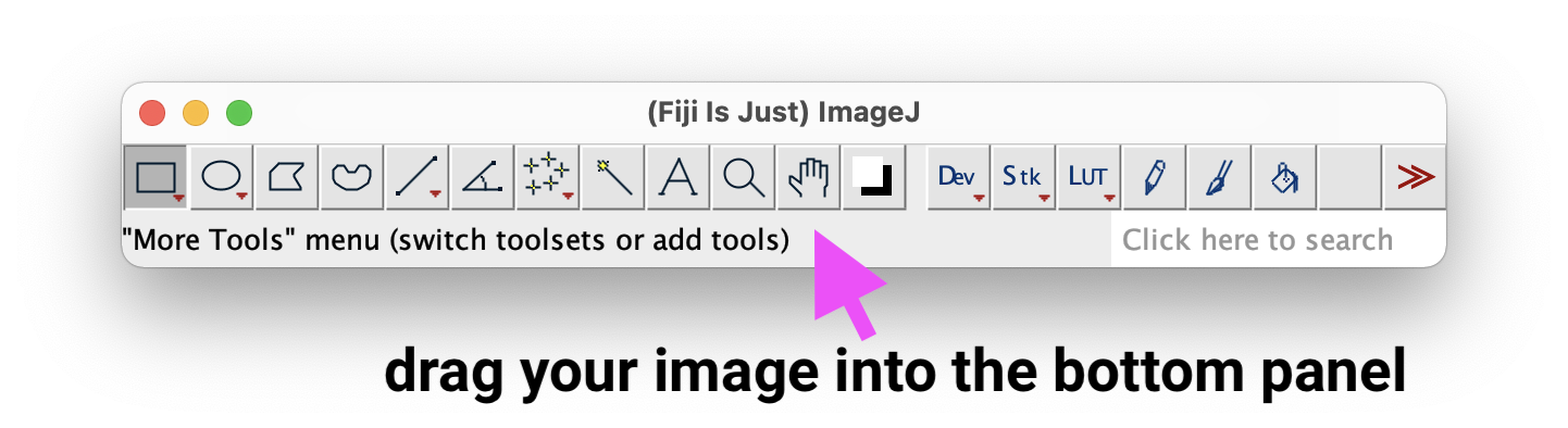
or open it via File > Open...

Note: The provied image files are already registered, i.e., corrected for movement artifacts. How to perform an image registration with Fiji can be, e.g., seen in this blog post ꜛ by Akira Muto.

2. Enhance the brightness settings

Enhance the visibility of the image by adjusting its brightness settings via Image > Adjust > Brightness/Contrast to open the B&C adjustment window. Either choose Auto or adjust appropriate brightness settings via the sliders:

3. Identify responding cells and z-project the image

To get an impression of which cells responded (i.e., show activity), move the slider at the bottom of the image window:

Next, we calculate the standard deviation of the image through all frames. Choose Image > Stacks > Z Project ...: which opens the ZProjection window:

Keep the default Start and Stop values, but change the Projection type to Standard Deviation. Press OK and the z-projected image appears in a new window:

4. Setting ROI in the z-projected image

Now we set regions of interest (ROI) on the identified responding cells.

First, let’s open the ROI Manager via Analyze > Tools > ROI Manager ... or press the key t:

Choos a selection tool from the main Fiji window, e.g., *Oval*,

and draw a ROI around a responding cell:

To add more ROI, press the Add [t] button in the ROI Manager or, again, press the key t. Repeat this step after each drawn ROI (otherwise your last drawn ROI won’t be saved in the ROI Manager).

Tip: For convenience, check the Show All box in the ROI Manager to see all drawn ROI.

After adding some ROI, your image might look similar to this:

5. Transfer the drawn ROI to the original image stack

Now, we save the ROI and re-open them in the original time lapse image stack.

In the ROI Manager, click on More and choose Save... and save the ROI file:

Click on the original time lapse image. In the ROI Manager, click again on More, but now choose Open... to import the previously saved ROI file (RoiSet.zip):

6. Measure and extract the mean pixel values of the ROI

In the main Fiji window, choose Analyze > Set Measurements ... to open the Set Measurements window. Check Mean gray value and uncheck all others:

Press OK.

In the ROI Manager, click again on More and choose Multi Measure. In the Multi Measure window, just click OK:

Fiji starts to slide through all image frames and extracts the brightness values of each drawn ROI. Once done, a Results table opens up:

Perform a right-click into the table and select Save As.... Save the table a CSV file (Results.csv).

7. Open the CSV file in your spreadsheet tool

Import the saved CSV file in the spreadsheet tool of your choice:

Please, note that the file is a comma-separated table, i.e., depending on your spreadsheet program, you can choose Open/Open with..., Import, or something similar. Then follow the provided instructions.
Another property of the file is, that the floating number separator is a . and not a , (which is common, e.g., for German numbers). If your spreadsheet tool is not in US or GB settings, account for this or change the language settings of your tool. Here is an example for Google Sheets:

In fact, it doesn’t matter if your spreadsheet tool will misinterpret the floating point separator. If it fails, the numbers become larger as they really are. Since we will continue to work with relative values, this won’t affect our results.

Here is an example import with Excel:

7. Estimate the background fluorescence

We now estimate the background fluorescence $F_0$ by averaging the lowest 25 % fluorescence values of each ROI. The following steps are examples for the procedure in Excel.

First, fix (“freeze”) the first row of the imported table:

Duplicate the first Excel sheet and sort all entries in ascending order:

Create a new sheet and set the first cell of the second column equal to the following formula (all formulas are provided for Englisch (left) and German (right) language settings):

=AVERAGE('Tabelle1 (2)'!B2:B501) or =MITTELWERT('Tabelle1 (2)'!B2:B501)

Transfer this formula to the remaining columns.

Explanation: The formula above calculates the average of the lowest 500 values per column (i.e., ROI or cell). They are the 500 lowest values, as we have sorted Tabelle1 (2) in ascending order. And since we have in total 2000 values (i.e., frames), we have indeed calculated the lowest 25 % of all brightness values per cell. By averaging this sub-set we estimate the background fluorescence $F_0$ of each cell.

8. Calculate the relative fluorescence changes

Let’s calculate the relative fluorescence change

\[F_\text{rel}(t) = \frac{\Delta F(t)}{F_0} = \frac{F(t) - F_0}{F_0}.\]

Again, create a new sheet and set the first cell of the second column equal to the following formula:

=(Tabelle1!B2 - Tabelle3!B$1)/Tabelle3!B$1

and transfer this formula to all 2000 rows and the remaining columns.

9. Adjust the time index

The time lapse was recorded with a frame rate of 16.6 fps. Set the first cell of column A to the formula:

=Tabelle1!A2/16,6

transfer this formula to all 2000 rows of this column.

10. Create a diagram

Create a diagram of all $F_\text{rel}(t)$ values of each cell. Set as x-axis values the values of column A:

Final remarks

While this tutorial demonstrates a straigh-forward way (i.e., with a minimum of required resources, that are all freely available) of extracting Ca²⁺ signals from time lapse image stacks, there are also more sophisticated solutions, which perform the extraction as well as the analysis fully or semi-fully automatic. State-of-the-art solutions are:

The CaImAn analysis pipeline:
- Paper ꜛ
- Documentation and installation instruction ꜛ (Python)
The suite2p analysis pipeline:
- Paper ꜛ
- Documentation and installation instruction ꜛ (Python)
- GitHub ꜛ

To quickly assess your data without having established one of these pipeline tools in your lab, you can apply some basic and self-written Python scripts to get already a first impression of your data in the extracted ROI table ꜛ. The following example code generates overview plots and statistical descriptions and performs a simple peak detection for spiking events:

import matplotlib.pyplot as plt
import pandas as pd
from scipy.signal import find_peaks
import os

# Import the Excel file:
file_path = "Data/Pandas_2/"
file_name = "ROI_table.xlsx"
sheet_to_read = "Tabelle1"
file = os.path.join(file_path, file_name)
ROI_df = pd.read_excel(file, index_col=0, sheet_name=sheet_to_read)

# Calculate from absolute to relative fluorescence changes by
# estimating the background fluorescence by calculating the average
# of the 25% lowest values per ROI:
N_rows = ROI_df.shape[0]
for ROI in ROI_df.keys():
    ROI_df[ROI] = (ROI_df[ROI] - ROI_df[ROI].sort_values().values[0:round(N_rows*0.25)].mean()) \
                / ROI_df[ROI].sort_values().values[0:round(N_rows * 0.25)].mean()

# Convert the index, i.e., time axis, into the appropriate scaling:
fps = N_rows / 120
ROI_df.index = ROI_df.index / fps

# Plot an overview of all ROI:
fig = plt.figure(1, figsize=(15,5))
fig.clf()
# ROI_df.plot()
for ROI in ROI_df.keys():
    plt.plot(ROI_df.index, ROI_df[ROI], lw=0.5, label=ROI, alpha=0.5)
plt.xlim((0,120))
# plt.legend()
plt.xlabel("time [s]")
plt.ylabel("$F_{rel}(t)$ [%]")
plt.title("Relative fluorescence changes of $Ca^{+2}$ signals")
plt.tight_layout()
plt.show()
plt.savefig("ROI_plot_all.png", dpi=90)

# Plot a ROI sub-set:
ROI_selection = [ "Mean20", "Mean28", "Mean30"]
spike_threshold=0
df_out = pd.DataFrame()

fig = plt.figure(2, figsize=(15,5))
fig.clf()
for ROI in ROI_selection:
    plt.plot(ROI_df.index, ROI_df[ROI], lw=0.75, label=ROI)

    # simple peak detection:
    current_spike_mask, _ = find_peaks(ROI_df[ROI],
                                       height=spike_threshold,
                                       prominence=0.5)
    plt.plot(ROI_df.index[current_spike_mask],
             ROI_df[ROI].iloc[current_spike_mask], '.', ms=10)
    df_out = pd.concat([df_out,
                        pd.DataFrame(ROI_df.index[current_spike_mask].values,
                                     columns=["ROI_"+str(ROI)])], axis=1)
plt.xlim((0,120))
plt.legend()
plt.xlabel("time [s]")
plt.ylabel("$F_{rel}(t)$ [%]")
plt.title("Relative fluorescence changes of selected $Ca^{+2}$ signals")
plt.tight_layout()
plt.show()
plt.savefig("ROI_plot_selected.png", dpi=90)

# Save some results tables:
ROI_df[ROI_selection].describe().to_excel("ROI selected stats.xlsx")
df_out.to_excel("ROI selected spike times.xlsx")

Plot of the relative fluorescence changes of all ROI:

Plot of the relative fluorescence changes of a ROI selection:

Desciptive statistics ꜛ of the ROI selection:

	Mean20	Mean28	Mean30
count	2000	2000	2000
mean	0,375523	0,249651	0,172436
std	0,453232	0,290448	0,162914
min	-0,2359	-0,2018	-0,26523
25%	0,099919	0,088341	0,075196
50%	0,25752	0,202324	0,155109
75%	0,482689	0,333547	0,241257
max	2,985423	2,431489	1,108501

Detected spike event times ꜛ in the ROI selection:

	ROI_Mean20	ROI_Mean28	ROI_Mean30
0	3,66	6,72	12,54
1	7,02	14,34	15,96
2	11,1	18,24	50,76
3	16,14	18,78	66,48
4	25,56	22,68	69,72
5	27,36	25,44	75,6
6	28,98	27,48	77,22
7	29,76	35,04	80,1
8	37,98	38,46	90,66
9	40,68	42,42	111,6
10	45,78	51,78	115,56
11	47,76	55,56	117,48
12	55,62	61,86
13	57,9	62,58
14	59,82	65,22
15	60,72	67,62
16	64,98	71,76
17	66,36	73,86
18	70,5	75,96
19	72,48	84,72
20	77,16	87,24
21	92,64	88,5
22	95,1	92,7
23	96,84	102,9
24	98,7	107,82
25	101,58
26	108,66
27	111,96
28	112,8
29	119,04

You could now continue, e.g., with the last table and calculate the average spike frequency per cell. You can also change the Python script in that way that it also extracts the spike amplitudes or calculates the average spike duration.

Acknowledgments

The presented tutorial is based on the online tutorial by Akira Muto ꜛ.

The data sets used in this tutorial are from:

M0_2017-10-13_003.tif: The suite2p GitHub repository ꜛ
Sue_2x_300040-46.tif: The CaImAn demo data-set ꜛ