Analyzing patch clamp recordings

In this chapter, we learn how to read patch clamp recordings from WaveMetrics IGOR ꜛ *.ibw files.

Short introduction to Patch Clamping

Patch clamp electrophysiology is a technique to examine ion channel behavior. Its subject is the study of ionic currents in individual isolated cells or patches of a cell membrane, both in-vivo and in-vitro.

To obtain a patch clamp recording, a so-called micropipette, a hollow glass tube filled with an electrolyte solution and a recording electrode connected to an amplifier, is used to form a seal with the memabrane of an isolated cell (see Fig. 1). A patch of a desired ion channel on the sealed cell membrane portion is removed or ruptured to enable electrical access to the cell. As a grounding reference, another electrode is placed in a bath surrounding the tissue, that contains the cell. This enables an electrical circuit between the grounding and the recording electrode. The recording can be performed in two modes:

• As a voltage clamp ꜛ: The voltage across the cell membrane is controlled by the amplifier, the resulting currents are recorded.
• As a current clamp ꜛ: The current passing across the membrane is controlled by the amplifier, the resulting voltage changes are recorded (in form of action potentials, see Fig. 2, right).

These two modes are used to study how ion channels behave both in normal and disease states and how these conditions can be modified, e.g., by drugs or other treatments.

Figure 1: Left: Schematic of a classical patch clamp recording setup (source: commons.wikimedia.org). Right: Schematic of a cell-attached patch clamp (source: commons.wikimedia.org).

Figure 2: Left: A patched cell viewed under the microscope (source: commons.wikimedia.org). Right: Example recording (bottom panel) and corresponding stimulation (here: optogentical, top panel) of a patched cell in an in-vitro probe (source: commons.wikimedia.org).

Figure 3: A classical patch clamp recording setup (source: commons.wikimedia.org).

Acknowledgement: The information within this section is gathered from the Wikipedia article on patch clamping ꜛ.

Preparations

Please install the following two packages with the Anaconda packages manager:

• neo (neuralensemble.org/neo, Paper ꜛ)
• igor (pypi.org/project/igor)

and download the following data from the GitHub repository:

• Data/Igor_1
• Data/Igor_2

Exercise 1

1. Create a new script, that reads in all IGOR binary ibw-files into a variable called, e.g., filenames. Hint: You can use the method we have introduced in the chapter Python pipeline for a basic time series analysis. Print out all read filenames.
2. Use the function sorted to sort the filenames in ascending order. Hint: Look-up the usage of sorted e.g. on python.org or realpython.com. What do you notice?

# Your solution 1.1-1.2 here:

file list (sorted): ['ad1_1.ibw', 'ad1_10.ibw', 'ad1_11.ibw', 'ad1_12.ibw', 'ad1_13.ibw', 'ad1_14.ibw', 'ad1_15.ibw', 'ad1_2.ibw', 'ad1_3.ibw', 'ad1_4.ibw', 'ad1_5.ibw', 'ad1_6.ibw', 'ad1_7.ibw', 'ad1_8.ibw', 'ad1_9.ibw']

Toggle solution

# Solution 1.1-1.2:
import numpy as np
import matplotlib
import pandas as pd
import matplotlib.pyplot as plt
import os
from neo import io

file_path = "Data/Igor_1/"
file_names = [file for file in os.listdir(file_path) \
              if file.endswith('.ibw')]
file_names = sorted(file_names)
print(f"file list (sorted): {file_names}")

Let’s see how the IGOR files look like:

test_file = os.path.join(file_path, file_names[0])
test_igor_read = io.IgorIO(test_file).read_analogsignal()

Please try out the following commands in your console, one after another:

test_igor_read

AnalogSignal with 1 channels of length 80000; units dimensionless; datatype float32
name: 'ad1_1'
annotations: {'note': b'WAVETYPE=adc \rTIME=12:47:40\ rComments=\rTemperature=0 \rBASELINE=-70.523515 \rBASESUBTRACTED=0.000000 \rREJECT=0.000000 \rSTEP=0.000000'}
sampling rate: 100.0 1/s
time: 0.0 s to 800.0 s

test_igor_read.shape

(80000, 1)

test_igor_read.sampling_rate

array(100.) * 1/s

np.array(test_igor_read.sampling_rate) # 1/s

array(100.)

test_igor_read.times

array([0.0000e+00, 1.0000e-02, 2.0000e-02, ..., 7.9997e+02, 7.9998e+02, ` 7.9999e+02]) * s`

Exercise 2

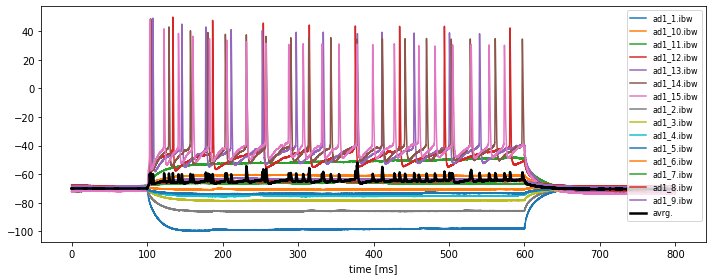
1. Iterate over all filenames and read each IGOR file by using the following command:

   current_igor_read = io.IgorIO(filepath).read_analogsignal()

   Plot each read IGOR trace into one figure by plotting current_igor_read.times vs. current_igor_read. Save this figure to disk. Adjust an appropriate figure aspect ratio and provide useful labels and legends.

2. In order to plot the average of all traces, we need to store each individual trace into a 2D numpy array, e.g. called all_igor_reads. Please recap our corresponding solution from Chapter 2.4, Python pipeline for a basic time series analysis and apply it to the current problem. Then calculate the grand average over all traces within the same figure.

# Your solution 2.1 and 2.2 here:

Toggle solution

# Solution 2.1 and 2.2:
all_igor_reads = np.empty((test_igor_read.shape[0], 0))

fig = plt.figure(1, figsize=(10,4))
plt.clf()
# for i, file in enumerate(file_names):
for file in file_names:

    current_file = os.path.join(file_path, file)
    current_igor_read = io.IgorIO(current_file).read_analogsignal()

    all_igor_reads = \
      np.append(all_igor_reads, current_igor_read.as_array(), axis=1)

    """ You can calculate the time-array manually,

    current_sampling_rate=np.array(current_igor_read.sampling_rate)
    current_time_array = np.arange(current_igor_read.shape[0]) /
                            current_sampling_rate
    plt.plot(current_time_array, current_igor_read, label=file)

    or use the .times attribute of the read-in igor file:
    """
    plt.plot(current_igor_read.times, current_igor_read, label=file)

plt.plot(current_igor_read.times, all_igor_reads.mean(axis=1), lw=2.5, c="k", label="avrg.")
plt.xlabel("time [ms]")
plt.legend(loc="best",fontsize=8)
plt.tight_layout()
#plt.show()
plt.savefig(file_path + " overview.pdf")

Exercise 3

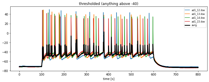
In order to kick-out traces without signifcant action potential spikings, we need to threshold the data:

• copy your solution from 2.1 and 2.2 into a new cell.
• rename the variable all_igor_reads into, e.g., thresholed_igor_reads and define a threshold kick_out_threshold = -40.
• change the plotting procedure in that way, that only traces with a maximum magnitude above kick_out_threshold are plotted.
• store these thresholded traces into the array thresholed_igor_reads.

# Your solution 3 here:

>>>
['ad1_12.ibw', 'ad1_13.ibw', 'ad1_14.ibw', 'ad1_15.ibw']

Toggle solution

# Solution 3
thresholed_igor_reads = np.empty((test_igor_read.shape[0], 0))
thresholed_igor_names = []
kick_out_threshold = -40

fig = plt.figure(2, figsize=(10, 4))
plt.clf()
# for i, file in enumerate(file_names):
for file in file_names:

    current_file = os.path.join(file_path, file)
    current_igor_read = io.IgorIO(current_file).read_analogsignal()

    #print(current_igor_read.shape)
    # thresholding:
    if np.max(current_igor_read) >= kick_out_threshold:
    #if np.mean(current_igor_read.as_array()[3000:15000]) >= kick_out_threshold:
        plt.plot(current_igor_read.times, current_igor_read, 
                 label=file)

        thresholed_igor_reads = np.append(thresholed_igor_reads, 
                                          current_igor_read.as_array(), 
                                          axis=1)
        #thresholed_igor_reads_times = np.append(thresholed_igor_reads_times, 
        #                              current_igor_read.times)
        thresholed_igor_names = thresholed_igor_names + [file]


plt.plot(current_igor_read.times, thresholed_igor_reads.mean(axis=1), lw=2.5, c="k", label="avrg.")
plt.xlabel("time [s]")
plt.title(f"thresholded (anything above {kick_out_threshold})")
plt.legend(fontsize=8)
plt.tight_layout()
plt.savefig(file_path + " overview thresholded.pdf")
plt.show()
print(thresholed_igor_names)

Exercise 4

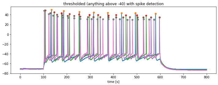
In order to detect the prominent spikes in each trace, we will apply the find_peaks function from the scipy package:

• please make yourself familiar with the find_peaks function on scipy.org.
• create a new cell and apply the find_peaks function to the previously thresholded traces stored in thresholed_igor_reads. Define a minimum threshold for the peak detection of spike_threshold = -10.

# Your solution 4 here:

Empty DataFrame
Columns: []
Index: []

Toggle solution

# Solution 4
from scipy.signal import find_peaks

spike_threshold = -10

df_out = pd.DataFrame() # initiliaze an empty Pandas DataFrame
print(df_out)

fig = plt.figure(3, figsize=(10, 4))
plt.clf()
for trace in range(thresholed_igor_reads.shape[1]):

    current_spike_mask, _ = find_peaks(thresholed_igor_reads[:,trace],
                                       height=spike_threshold)

    plt.plot(current_igor_read.times,
             thresholed_igor_reads[:, trace].flatten())

    plt.plot(current_igor_read.times[current_spike_mask],
             thresholed_igor_reads[current_spike_mask, trace].flatten(), '.', ms=10)

    # Now, we fill our empty DataFram with the peak-time points
    #   of each trace:
    df_out = pd.concat([df_out, 
                        pd.DataFrame(current_igor_read.times[current_spike_mask], 
                                    columns=[thresholed_igor_names[trace]])],
                       axis=1)
    
    #print(f"peak times: {current_igor_read.times[current_spike_mask]}")

plt.xlabel("time [s]")
plt.title(f"thresholded (anything above {kick_out_threshold}) with spike detection")
plt.tight_layout()
plt.savefig(file_path + " overview thresholded and spikes.pdf")
plt.show()

# at the end, let's save our new DataFrame as an Excel-File:
df_out.to_excel("my_peaks.xlsx")

The extracted parameters from this time series can be used for further analysis. For instance, from the detected peaks you could calculate the peak frequency. Also, you could further extract the peak amplitudes and calculate the average peak magnitude or assess magnitude variations.

Outlook: We will learn other methods to extract the peak frequency in the chapter about Fourier Transformation.

Exercise 5

The folder Data/Igor_2 contains the corresponding stimulation steps of the recorded action potentials from Data/Igor_1 that we have analyzed so far.

1. Read the data from the Data/Igor_2 folder.
2. Apply a new thresholding method to the recorded and so far analyzed action potentials: Instead of applying a hard threshold (kick_out_threshold = -40), now exclude all patch clamb recordings whose corresponding stimulation was negative.

# Your solution 5 here:

References

• Wikipedia article ꜛ on patch clamping
• Wikipedia article ꜛ on voltage clamping
• Wikipedia article ꜛ on current clamping
• Purves D, Augustine GJ, Fitzpatrick D, et al., editors. Neuroscience. 2nd edition. Sunderland (MA): Sinauer Associates; 2001. Box A, The Patch Clamp Method. Available from: ncbi.nlm.nih.gov
• Segev A, Garcia-Oscos F, Kourrich S. Whole-cell Patch-clamp Recordings in Brain Slices. J Vis Exp. 2016;(112):54024. Published 2016 Jun 15. doi:10.3791/54024, read free on PubMed link ꜛ
• The Nobel Prize in Physiology or Medicine 1991. nobelprize.org, Nobel Media AB. Retrieved: August 30, 2021