Distinguishing correlation from the coefficient of determination: Proper reporting of r and R²

I noticed that people sometimes report $R^2$ – “R-squared” – instead of the Pearson correlation coefficient $r$ when discussing the correlation between two variables. In the special case of a simple linear relationship this numerical equality is not strictly wrong, yet presenting $R^2$ as if it were the correlation coefficient might wrongly give the impression they are the same thing. In this post, we will therefore unpack the difference between these two measures, explain their mathematical definitions and proper usage discuss the best practices for when to use each in statistical reporting.

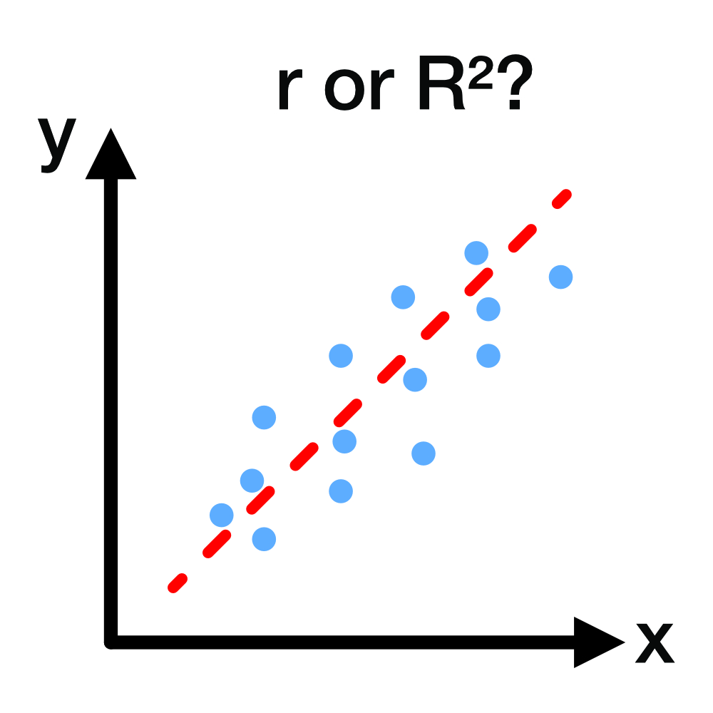
When to report $r$ vs $R^2$: $r$ quantifies the strength and direction of linear association between two variables, while $R^2$ measures the proportion of variance explained by a regression model. In this post, we clarify their definitions, relationship, and appropriate contexts for use.

What is correlation?

Correlation is a statistical measure used across many fields, from neuroscience to physics and economics, to quantify the linear association between two variables, or, put simply, how they change together. Imagine plotting paired measurements as points on a scatter plot. Now suppose the points seem to cluster along an imagined straight line. If this imagined line points upward, the two measurements “correlate”, i.e., they vary together in a consistent way. If the line points downward, the two measurements vary inversely, i.e., they are anti‑correlated, meaning they vary in opposite directions. If the best-fit line is approximately horizontal and the points show no overall trend, there is (almost) no correlation. Mathematically, correlation is defined without requiring a fitted line — the line is just a visualization aid. If the points instead form a diffuse cloud with no clear trend and no meaningful line can be drawn, this likewise indicates no correlation, i.e., the two measurements change independently of each other.

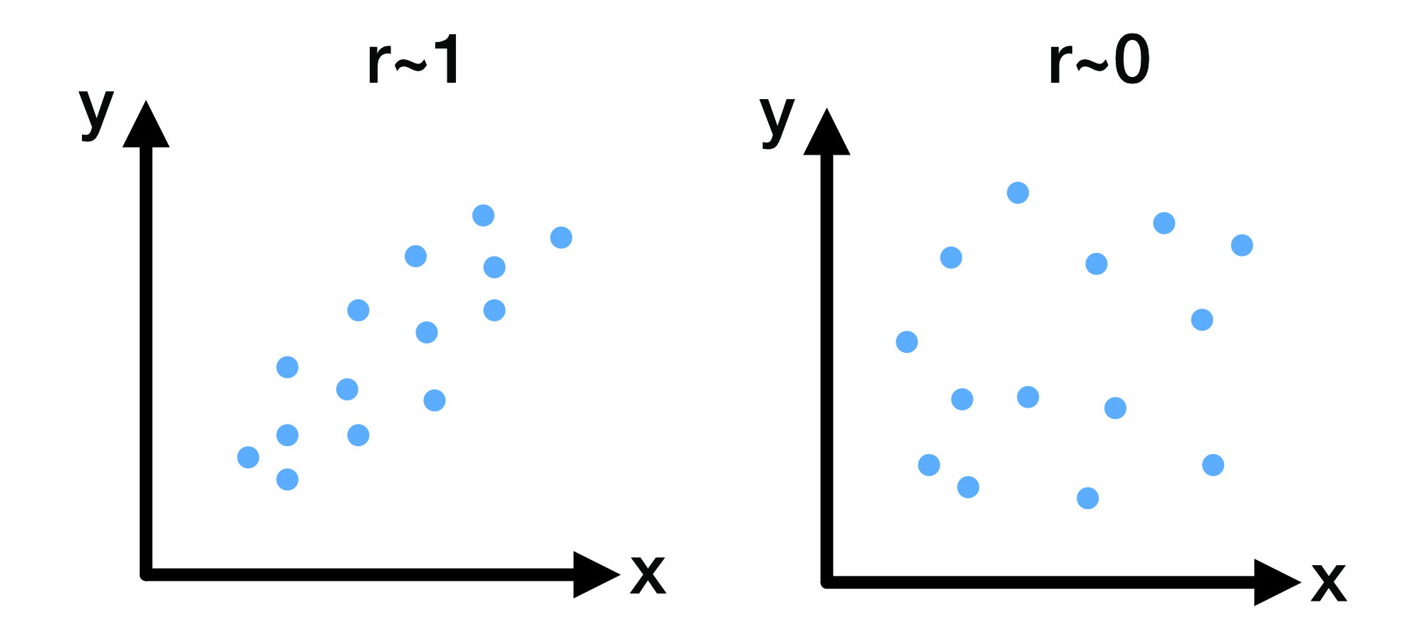Example scatterplots illustrating correlation strength: left, a strong positive linear association ($r \approx 1$); right, no linear association ($r \approx 0$).

To assess the degree of correlation, there are different metrics. The most common one is the Pearson correlation coefficient $r$, named after Karl Pearson, who introduced and rigorously formalized the concept of the correlation coefficient in the late 19th century. The value of $r$ is close to $+1$ when two measurements are strongly positively correlated. If $r$ is close to $−1$, the measurements are strongly negatively correlated (anti‑correlated). When $r$ is near $0$, the measurements show little or no linear association. These values capture both the strength (value) and the direction (sign) of the relationship between two variables.

Mathematical definition of the Pearson correlation coefficient

The Pearson correlation can be seen as a normalized measure of how two variables co-vary: the covariance $\operatorname{cov}(X,Y)$ describes their joint variability, and dividing by their standard deviations produces a unitless coefficient.

For random variables $X$ and $Y$ with means $\mu_X,\mu_Y$ and standard deviations $\sigma_X,\sigma_Y$, the population (Pearson) correlation is:

\[\begin{align*} \rho_{XY} =& \frac{\operatorname{cov}(X,Y)}{\sigma_X \sigma_Y} \\ =& \frac{\mathbb{E}\!\big[(X-\mu_X)(Y-\mu_Y)\big]}{\sigma_X \sigma_Y} \end{align*}\]

$\mathbb{E}[\cdot]$ denotes expectation.

For a sample ${(x_i,y_i)}_{i=1}^n$ with $x_i, y_i$ the paired measurements, sample means $\bar x,\bar y$ and sample standard deviations $s_X,s_Y$, the sample correlation is

\[\begin{align*} r =& \frac{\sum_{i=1}^n (x_i-\bar x)(y_i-\bar y)} {\sqrt{\sum_{i=1}^n (x_i-\bar x)^2}\,\sqrt{\sum_{i=1}^n (y_i-\bar y)^2}}\\ =& \frac{\operatorname{cov}_{\text{sample}}(X,Y)}{s_X s_Y} \end{align*}\]

where

\[\operatorname{cov}_{\text{sample}}(X,Y)=\frac{1}{n-1}\sum_{i=1}^n (x_i-\bar x)(y_i-\bar y),\] \[s_X^2=\frac{1}{n-1}\sum_{i=1}^n (x_i-\bar x)^2,\]

and

\[s_Y^2=\frac{1}{n-1}\sum_{i=1}^n (y_i-\bar y)^2\]

are the sample covariance and sample variances, respectively. The terms $(x_i-\bar x)$ and $(y_i-\bar y)$ are called mean-centered values because the sample means $\bar x$ and $\bar y$ have been subtracted from each data point. This centering ensures that the correlation measures how deviations from the mean in one variable relate to deviations from the mean in the other variable. The division by $s_X$ and $s_Y$ normalizes the covariance, making $r$ a dimensionless quantity that is independent of the units of measurement of $X$ and $Y$. This normalization allows for meaningful comparisons of correlation strength across different datasets

Notice that the sample covariance and the sample variances each include a factor of $1/(n-1)$. When you substitute these definitions into the fraction for $r$, the $1/(n-1)$ in the numerator and the two $1/(n-1)$ factors under the square roots in the denominator cancel out. That is why the commonly used summation formula for $r$ does not explicitly contain $1/(n-1)$.

An equivalent expression in terms of standardized z-scores $z_{Xi}=(x_i-\bar x)/s_X$ and $z_{Yi}=(y_i-\bar y)/s_Y$ is

\[r = \frac{1}{n-1}\sum_{i=1}^n z_{Xi}\,z_{Yi}\]

This formulation makes clear that $r$ is just the average product of paired standardized values.

$r$ inherits several important properties: by the Cauchy–Schwarz inequality, $r$ always lies between −1 and +1: $r\in[-1,1]$. Furthermore, $r$ is dimensionless and remains unchanged if either variable is shifted by a constant or scaled by a positive factor (a negative scaling factor only flips its sign).

In many applied sciences, rough guidelines are sometimes used to describe correlation strength: values of about

• $|r| \ge 0.7$ are often called strong,
• $|r| \approx 0.3$–$0.7$ moderate, and
• $|r| \le 0.3$ weak or negligible.

The sign of $r$ indicates the direction of association (positive or negative). These thresholds are not universal: they vary by field, sample size, and context. Thus, they should be interpreted cautiously.

Alternatives to Pearson correlation

When two variables change together in a consistent, i.e., monotonic way but their relationship is not linear, or when the data are ordinal or contain outliers, rank-based measures are often more appropriate:

Spearman’s rank correlation ($\rho_s$)
Spearman replaces each raw value with its rank in the sorted data.

Let $R_i$ be the rank of the $i$-th value of the first variable and $S_i$ the rank of the corresponding value of the second variable (average ranks are used for ties). Let $\bar R$ and $\bar S$ be the average ranks (for data without ties, both equal $(n+1)/2$). Two perfectly monotonic relationships — one always increasing, one always decreasing — will produce $\rho_s$ values of +1 or −1 even if the points do not line up linearly. Spearman’s $\rho_s$ is then computed just like a Pearson correlation, but on these ranks:

\[\rho_s = \frac{\sum_{i=1}^n (R_i-\bar R)(S_i-\bar S)}{\sqrt{\sum_{i=1}^n (R_i-\bar R)^2}\,\sqrt{\sum_{i=1}^n (S_i-\bar S)^2}}.\]

Without ties, the common shortcut applies:

\[\rho_s = 1 - \frac{6\sum d_i^2}{n(n^2-1)}, \quad d_i = R_i-S_i.\]

Kendall’s tau ($\tau$)
Kendall’s method works by examining all possible pairs of observations. For any two points $(x_i,y_i)$ and $(x_j,y_j)$, the pair is called concordant if the ordering of $x_i$ and $x_j$ agrees with the ordering of $y_i$ and $y_j$ (both increase or both decrease together). It is discordant if these orderings disagree (one increases while the other decreases).

Let $C$ be the total number of concordant pairs and $D$ the total number of discordant pairs among the $\binom{n}{2}$ possible pairs. Kendall’s tau is then defined as

\[\tau = \frac{C-D}{\binom{n}{2}}\]

This coefficient represents the difference between the proportions of concordant and discordant pairs, providing a robust measure of association for ordinal or non-normally distributed data and making it less sensitive to outliers than Pearson’s $r$.

These rank-based measures focus on the relative ordering of data rather than their actual values, making them robust to non-normal distributions and outliers. For relationships that are strong but non-monotonic (e.g., U-shaped), even these measures may be near zero; in such cases, distance correlation or mutual information can be considered.

Significance testing and confidence intervals for $r$

To determine whether an observed Pearson correlation $r$ differs significantly from zero, one typically uses a t-test under the null hypothesis $H_0:\rho=0$ (no linear association in the population). Under the assumption of bivariate normality, the test statistic is

\[t = r \sqrt{\frac{n-2}{1-r^2}}\]

with degrees of freedom $\mathrm{df}=n-2$, where $n$ is the number of paired observations. This $t$ value is compared to a $t$-distribution with $n-2$ degrees of freedom to compute a two-sided or one-sided p-value:

• A two-sided p-value answers: “Is the absolute value of $r$ unusually large if the true correlation is zero?”
• A one-sided p-value is used only if a specific direction of correlation (positive or negative) was pre-specified.

As $|r|$ approaches 1, the numerator grows and $t$ becomes large, indicating strong evidence against $H_0$. For small sample sizes, even moderate $r$ may not be significant because the denominator $1-r^2$ inflates $t$ less strongly.

Confidence intervals for $r$: Fisher z-transformation

The sampling distribution of $r$ is skewed, especially for values near $\pm 1$, which makes direct confidence intervals for $r$ inaccurate. To address this, Fisher’s z-transformation is applied:

\[z = \frac{1}{2}\ln\!\left(\frac{1+r}{1-r}\right) = \operatorname{arctanh}(r)\]

which approximately normalizes the distribution of $r$ for moderate $n$. The transformed variable $z$ has an approximate standard error

\[\mathrm{SE}_z = \frac{1}{\sqrt{n-3}}\]

A $(1-\alpha)$ confidence interval for $z$ is

\[z \pm z_{\alpha/2} \,\mathrm{SE}_z\]

where $z_{\alpha/2}$ is the critical value from the standard normal distribution (e.g., 1.96 for a 95% CI). Transform the endpoints back to the $r$ scale using the inverse transformation

\[r = \tanh(z) = \frac{e^{2z}-1}{e^{2z}+1}\]

This yields a confidence interval for the population correlation $\rho$ that is nearly symmetric on the $z$-scale but properly accounts for the skewness on the $r$-scale.

Introducing $R^2$ (coefficient of determination)

In linear regression, we are often interested in how well a straight line fits a cloud of data points. Suppose we model a response variable $y$ as a linear function of a single predictor $x$ plus random noise:

\[y_i = \beta_0 + \beta_1 x_i + \varepsilon_i,\quad i=1,\dots,n\]

Here, $\beta_0$ is the intercept, $\beta_1$ the slope, and $\varepsilon_i$ are residual errors assumed to have mean zero. The fitted values from least squares regression are

\[\hat y_i = \hat \beta_0 + \hat \beta_1 x_i\]

To evaluate the quality of this fit, we compare the variation in the data explained by the model to the total variation present in $y$. We decompose the total sum of squares (SST),

\[\mathrm{SST} = \sum_{i=1}^n (y_i - \bar y)^2,\]

into the regression sum of squares (SSR), representing the variability explained by the model,

\[\mathrm{SSR} = \sum_{i=1}^n (\hat y_i - \bar y)^2\]

and the residual sum of squares (SSE or sometimes SSR in other texts),

\[\mathrm{SSE} = \sum_{i=1}^n (y_i - \hat y_i)^2\]

The coefficient of determination, $R^2$, is then defined as the proportion of the variance in $y$ explained by the regression:

\[R^2 = 1 - \frac{\mathrm{SSE}}{\mathrm{SST}} = \frac{\mathrm{SSR}}{\mathrm{SST}}.\]

An $R^2$ of 1 indicates that all data points lie perfectly on the fitted line (the model explains all variation in $y$). An $R^2$ of 0 means the model explains none of the variability — using the mean $\bar y$ as a “model” is no worse than using $x$. Negative values of $R^2$ can occur if the chosen model fits worse than simply predicting $\bar y$ for all observations, which may happen in poorly specified regressions or with nonlinear relationships.

Conceptually, $R^2$ quantifies explained variance: it measures how much of the observed variation in the response variable can be attributed to variation in the predictor variable, under a linear least squares model.

How $r$ and $R^2$ are related

Consider simple linear regression with an intercept:

\[y_i = \beta_0 + \beta_1 x_i + \varepsilon_i\]

and let $\bar x,\bar y$ be sample means. Define the centered sums:

\[\begin{align*} S_{xx}=&\sum_{i=1}^n (x_i-\bar x)^2,\\ S_{yy}=&\sum_{i=1}^n (y_i-\bar y)^2,\\ S_{xy}=&\sum_{i=1}^n (x_i-\bar x)(y_i-\bar y) \end{align*}.\]

Using ordinary least squares (OLS), the standard method that minimizes the sum of squared residuals, the slope is

\[\hat\beta_1=\frac{S_{xy}}{S_{xx}}\]

and the Pearson correlation is

\[r=\frac{S_{xy}}{\sqrt{S_{xx}S_{yy}}}.\]

Hence

\[\hat\beta_1 = r\,\frac{\sqrt{S_{yy}}}{\sqrt{S_{xx}}}.\]

Fitted values satisfy $\hat y_i-\bar y=\hat\beta_1(x_i-\bar x)$, so the regression (explained) sum of squares is

\[\mathrm{SSR}=\sum_{i=1}^n (\hat y_i-\bar y)^2=\hat\beta_1^{\,2}\,S_{xx} = r^2\,S_{yy}\]

The total sum of squares is $\mathrm{SST}=S_{yy}$. Therefore

\[R^2=\frac{\mathrm{SSR}}{\mathrm{SST}}=\frac{r^2\,S_{yy}}{S_{yy}}=r^2\]

Key conditions and caveats:

• The identity $R^2=r^2$ holds only for simple linear regression with an intercept (one predictor, least squares, standard definitions).
• In models with multiple predictors or nonlinear terms, $R^2$ equals the squared correlation between the observed response and its fitted values, \(R^2=\operatorname{corr}(Y,\hat Y)^2,\) but it is not equal to the square of any single pairwise correlation (e.g., $\operatorname{corr}(X_j,Y)^2$).
• If the intercept is omitted (regression through the origin), the decomposition $\mathrm{SST}=\mathrm{SSR}+\mathrm{SSE}$ changes and the result $R^2=r^2$ need not hold.
• $R^2$ discards the sign of association: $r$ and $-r$ yield the same $R^2$. Thus, we lose information about the direction of the relationship when reporting only $R^2$. When reporting only $R^2$, one should also report the slope sign or $r$ to retain directionality.

When to report $r$ vs $R^2$

The Pearson correlation coefficient $r$ and the coefficient of determination $R^2$ serve different purposes and should be reported in contexts that match their meaning:

• For pure correlation questions, report $r$
  When the goal is to describe how two variables co-vary without fitting a predictive model, $r$ is the appropriate measure. It conveys both the strength (magnitude) and direction (sign) of the linear relationship. Reporting only $R^2$ would discard the sign and obscure whether the association is positive or negative.
• For model goodness-of-fit, report $R^2$
  In linear regression or more complex predictive models, $R^2$ quantifies explained variance, i.e., the proportion of variability in the response variable accounted for by the model. It is a natural summary of model performance and is meaningful even with multiple predictors or non-linear terms (as the squared correlation between observed and fitted values).
• If $R^2$ is used as a proxy for correlation, include directional information
  In some neuroscience and biology papers, $R^2$ is shown on scatterplots as a stand-in for correlation strength. This is not strictly wrong in simple linear relationships but can be misleading. To avoid ambiguity, also report the slope sign or $r$ itself so that the direction of association is not lost.

Using the right statistic in the right context prevents confusion: $r$ answers “how strongly and in which direction do these two variables co-vary?” whereas $R^2$ answers “how much of the variance in the response is explained by this model?”

Why the misconception persists

The confusion between $r$ and $R^2$ has multiple roots in practice and pedagogy:

• Teaching shortcuts
  In teaching, $R^2$ and $r^2$ are sometimes presented side by side without making it clear enough that the equality $R^2 = r^2$ holds only under specific conditions (single predictor, intercept included). Over time, this can lead students to internalize the idea that “$R^2$ is the correlation”, overlooking the assumptions behind the equivalence.
• Software defaults
  Analysis tools such as GraphPad Prism, Excel, and some statistical packages automatically report $R^2$ in correlation analyses. This can prompt users to treat $R^2$ as the default measure of linear association, especially if they are not fully aware of the distinction.
• Plotting conventions in applied sciences
  It is common to “fit a line to guide the eye” and annotate the plot with $R^2$. Although this is acceptable for assessing fit quality, it reinforces the misconception that $R^2$ alone suffices to describe correlation strength and direction.
• Simplicity and sign removal
  Some practitioners prefer $R^2$ because it is always non-negative and superficially “cleaner” to report. However, this very feature hides the direction of the relationship and can obscure scientific interpretation.

These teaching and software habits may explain why the misconception persists. Just to get me right, this is not meant as a blanket criticism of anyone’s work, only a reminder that common shortcuts can sometimes obscure important distinctions.

Simple Python examples

To get a better impression of the difference between $r$ and $R^2$, let’s look at some synthetic datasets with varying degrees of correlation. In the following, we will create six different toy datasets, which contain

• a strong positive correlation,
• a strong negative correlation,
• a moderate positive correlation,
• a moderate negative correlation,
• no correlation (data points cluster along a virtual horizontal line), and, again,
• no correlation (a random cloud of points).

Each dataset is superimposed with some Gaussian noise to simulate real-world variability. We will compute both $r$ and $R^2$ for each dataset and visualize the results:

# imports:
import numpy as np
import matplotlib.pyplot as plt
from scipy.stats import pearsonr
from sklearn.metrics import r2_score

# set global properties for all plots:
plt.rcParams.update({'font.size': 14})
plt.rcParams["axes.spines.top"]    = False
plt.rcParams["axes.spines.bottom"] = False
plt.rcParams["axes.spines.left"]   = False
plt.rcParams["axes.spines.right"]  = False

# set seed for reproducibility:
rng = np.random.default_rng(42)

# generate synthetic datasets:
n = 50
x = np.linspace(-3, 3, n)

# strong correlations
y_pos_strong = 2 * x + rng.normal(scale=1.0, size=n)
y_neg_strong = -2 * x + rng.normal(scale=1.0, size=n)

# moderate correlations (more scatter)
y_pos_moderate = 2 * x + rng.normal(scale=4.0, size=n)
y_neg_moderate = -2 * x + rng.normal(scale=4.0, size=n)

# no correlation cases
y_horiz = 0 + rng.normal(scale=1.0, size=n)
x_cloud = rng.uniform(-3, 3, size=n)
y_cloud = rng.uniform(-10, 10, size=n)  # oder rng.normal(scale=3, size=n)

datasets = [
    ("Strong pos. correlation", x, y_pos_strong),
    ("Strong neg. correlation", x, y_neg_strong),
    ("Moderate pos. correlation", x, y_pos_moderate),
    ("Moderate neg. correlation", x, y_neg_moderate),
    ("No correlation (horizontal)", x, y_horiz),
    ("No correlation (cloud)", x_cloud, y_cloud)
]

# plots:
fig, axes = plt.subplots(3, 2, figsize=(10, 16))
for ax, (title, xdata, ydata) in zip(axes.flat, datasets):
    r, _ = pearsonr(xdata, ydata)
    coeffs = np.polyfit(xdata, ydata, 1)
    y_fit = np.polyval(coeffs, xdata)
    r2 = r2_score(ydata, y_fit)

    ax.scatter(xdata, ydata, alpha=0.7)
    ax.plot(np.sort(xdata), np.polyval(coeffs, np.sort(xdata)),
            color='red', lw=2, label='Linear fit')
    ax.set_title(title)
    ax.set_xlabel('x')
    ax.set_ylabel('y')
    ax.legend()
    ax.text(0.05, 0.95, f"r = {r:.2f}\nR² = {r2:.2f}",
            transform=ax.transAxes, va='top', ha='left',
            bbox=dict(boxstyle='round', facecolor='white', alpha=0.7, lw=0))
    ax.set_xlim(-3,3)
    ax.set_ylim(-10,10)

plt.tight_layout()
plt.savefig('correlation_vs_rsquare.png', dpi=300)
plt.show()

In the strong correlation plots, both $r$ and $R^2$ are close to 1. The left panel shows a positive correlation, whereas the right panel shows a negative one. While $r$ retains the sign, indicating whether the relationship is positive or negative, this information is lost in $R^2$, which is always non-negative.

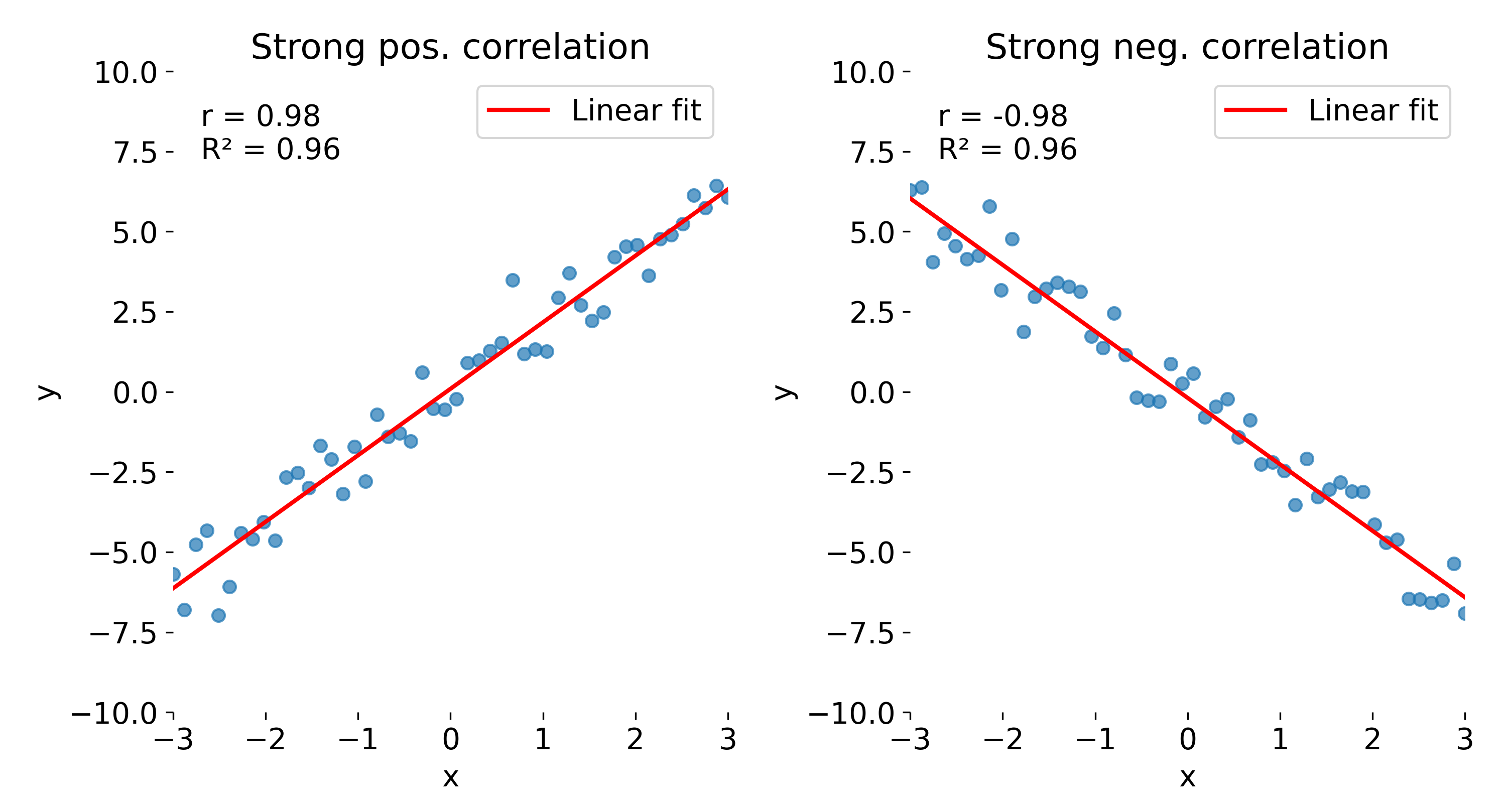Comparison of correlation coefficient ($r$) and coefficient of determination ($R^2$) across different datasets. Here, strong positive (left) and strong negative (right) correlations are shown.

With the next set of toy data, we repeat the same experiment but add more noise. As a result, both $r$ and $R^2$ decrease, reflecting the weaker linear association. Again, $r$ indicates the direction of the relationship, while $R^2$ does not.

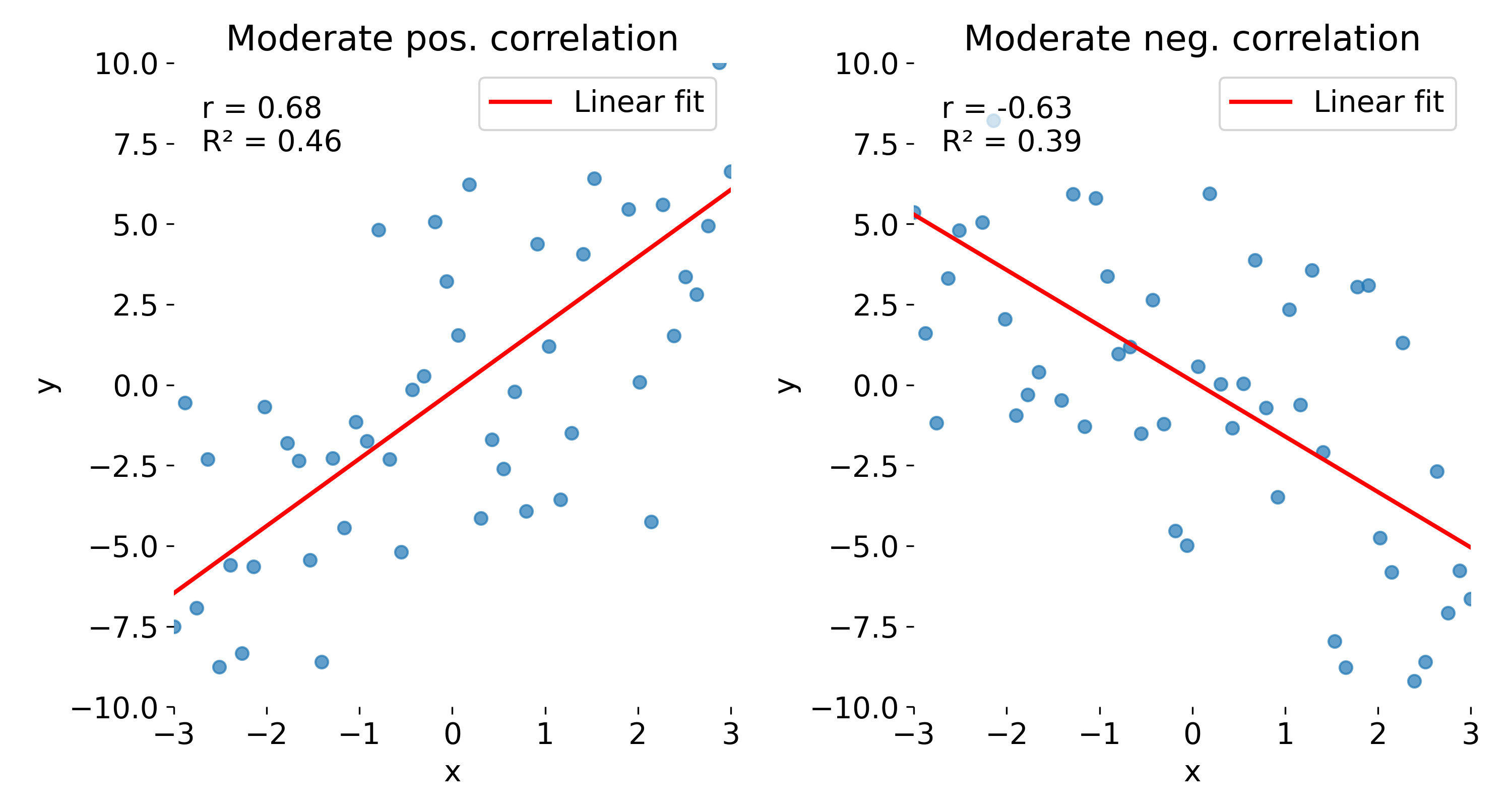Same plots as before, but now with moderate correlations due to increased noise. Left: moderate positive correlation; right: moderate negative correlation.

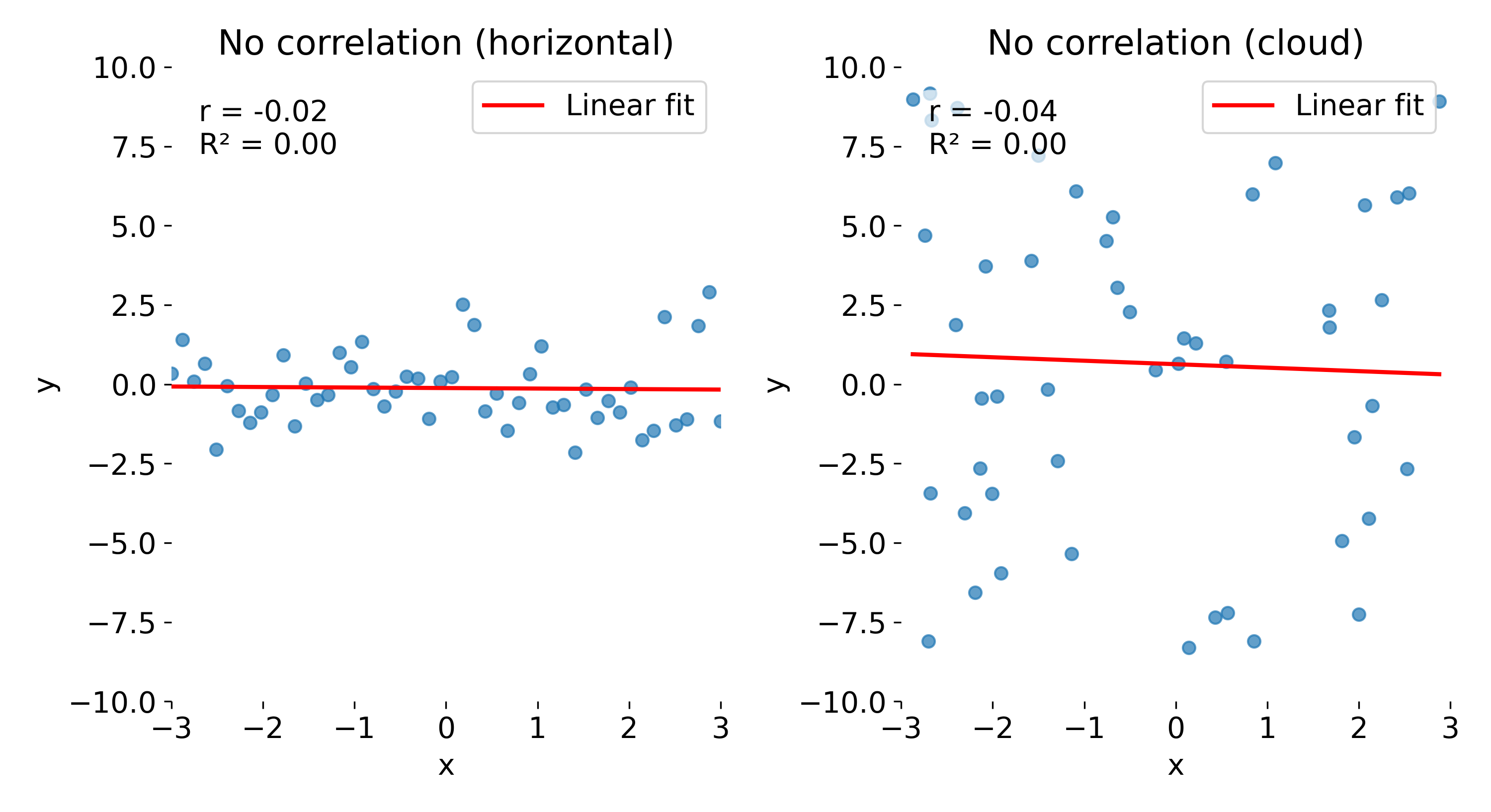
The last toy datasets illustrate cases with no correlation. In the first case (left panel), the data points cluster around a horizontal line. Here, $r$ is close to 0, indicating no linear association, and $R^2$ is also near 0, showing that the linear model explains almost none of the variance in $y$.

Same plots as before, but now with no correlation. Left: no correlation (horizontal line); right: no correlation (random cloud of points).

In the second panel (right), we see a random cloud of points with no discernible trend. Again, both $r$ and $R^2$ are close to 0, indicating no linear relationship. However, note that while the absolute variability in $y$ is much larger here than in the horizontal case, $R^2$ does not reflect this difference — it only indicates that there is no linear relationship between $x$ and $y$. Even if the data points show very different amounts of scatter, $R^2$ quantifies only the proportion of variance in $y$ explained by a linear relationship with $x$. A value of $R^2 = 0$ does not distinguish between a case where the data are nearly constant (small absolute variance) and a case where they are widely dispersed (large absolute variance); it merely indicates that none of this variance is linearly associated with $x$. This underscores another potential misconception: $R^2$ is not a direct measure of absolute variability in the data.

Conclusion

Correlation coefficients and coefficients of determination answer different questions. The Pearson correlation $r$ measures the strength and direction of a linear association between two variables, while $R^2$ quantifies the proportion of variance in the response that a linear regression model explains. Their numerical equality in simple linear regression ($R^2 = r^2$) is a special case, not a universal identity.

In practice, it is easy to slip into treating $R^2$ as the correlation. To avoid this trap, I’d suggest: for pure correlation analysis, i.e., when you are simply checking whether and how two variables co-vary, report $r$, because it preserves both the strength and the sign of the relationship. For model evaluation and goodness-of-fit, report $R^2$, which summarizes how much of the variance is accounted for by your regression model. And if you annotate scatterplots with $R^2$ as a visual guide, add the slope sign or $r$ as well, so that the direction of the relationship is not lost.

Finally, keep in mind that $R^2$ is not a measure of absolute variability in the data. A value of $R^2=0$ does not distinguish between tightly clustered points and widely dispersed clouds. It only says that no linear relationship exists.

Being clear about what $r$ and $R^2$ each convey helps avoid confusion and keeps your reporting transparent.

References

• David Freedman, Statistics, 2010, Viva Books, 4th edition, ISBN: 9788130915876
• Andrew Gelman, Jennifer Hill, Aki Vehtari, Regression And Other Stories, 2021, Cambridge University Press, ISBN: 9781107023987
• Bevington, P. R., & Robinson, D. K. Data reduction and error analysis for the physicals science, 2003, 3rd ed., McGraw-Hill, ISBN: 0-07-247227-8