Implementing a minimal spiking neural network for MNIST pattern recognition using nervos

I recently came across nervosꜛ, an open source spiking neural network framework recently developed by Jaskirat Singh Maskeenꜛ and Sandip Lashkareꜛ. nervos aims to provide a unified and hardware aware platform to evaluate different spike timing dependent plasticity learning rules together with different synapse models, ranging from idealized floating point synapses to finite state nonlinear memristor based models. The framework is described in A Unified Platform to Evaluate STDP Learning Rule and Synapse Model using Pattern Recognition in a Spiking Neural Networkꜛ.

In this post, we use nervosꜛ (Maskeen & Lashkare, 2025ꜛ) to implement a minimal two layer spiking neural network for pattern recognition on the MNIST dataset. We analyze how the network learns to classify digits through STDP and how the synaptic weights evolve during training. The figure shows the evolution of synaptic weights for a single output neuron over the course of training, illustrating how the network develops selectivity for certain input patterns corresponding to specific digit classes. We will further analyze the internal dynamics of the network, the learned receptive fields, and the classification performance on the test set. The code for this example is available in the Github repository mentioned at the end of this post.

I was curious and applied nervos to a classical pattern recognition task using MNIST digits. I basically replicated their original tutorial “MNIST Exampleꜛ” and then extended it with additional analyses. The goal was to understand in detail how a minimal two layer spiking network with purely local plasticity can self organize into digit selective neurons, how classification emerges, and what exactly is stored internally for later analysis. In this post, I summarize the mathematical formulation of the network, the learning rules, and the results I obtained.

Mathematics of nervos

Let’s first have a look at the mathematical formulation of the network architecture. In the following, we will walk through the main components of the model, including the network architecture, input encoding, neuron and synapse models, and the STDP learning rule. This is the best way to understand what the model does and how it learns, before we go ahead to the actual implementation and results.

Network architecture

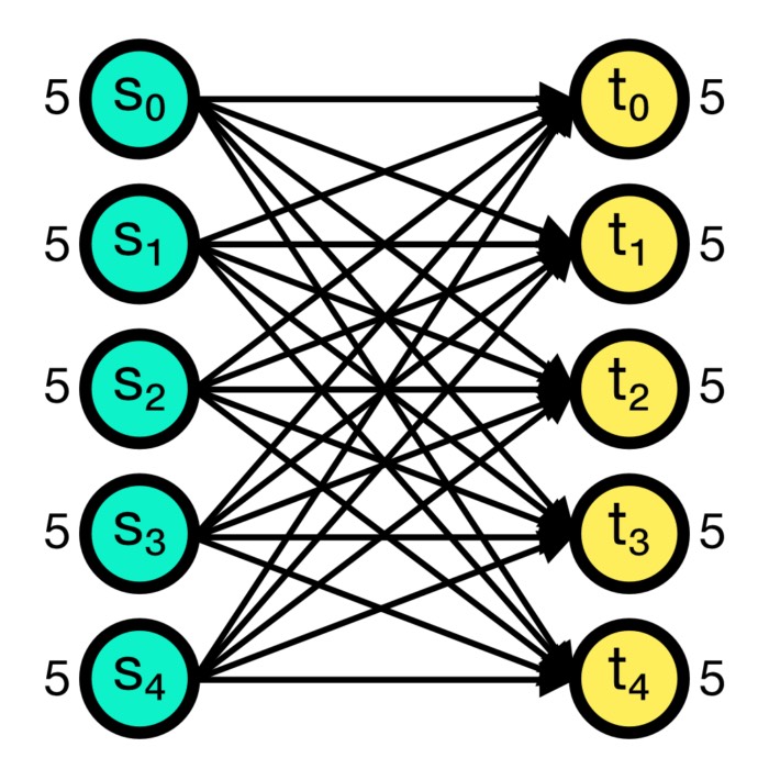
The architecture implemented in nervos is deliberately minimal. It consists of a two layer spiking neural network without hidden layers:

• Input layer: we will use 784 neurons corresponding to the 28×28 pixels of an MNIST imageꜛ.
• Output layer: typically 60 or 80 neurons depending on the experiment (we will use 80 in our example).

Every input neuron is connected to every output neuron via an excitatory synapse. Thus, the weight matrix is

\[W \in \mathbb{R}^{N_{\text{out}} \times 784},\]

with entries $w_{ij}$ representing the synaptic strength from input neuron $j$ to output neuron $i$, with $N_{\text{out}}$ being the number of output neurons.

Competition in the output layer is implemented algorithmically. At each time step, the neuron with the highest membrane potential is identified. If this neuron crosses its adaptive threshold, it emits a spike and all other neurons are inhibited by resetting their potentials to an inhibitory level and placing them into a refractory state. There is no explicit lateral inhibitory connectivity matrix; instead, Winner Takes All dynamics are enforced by this global inhibition rule.

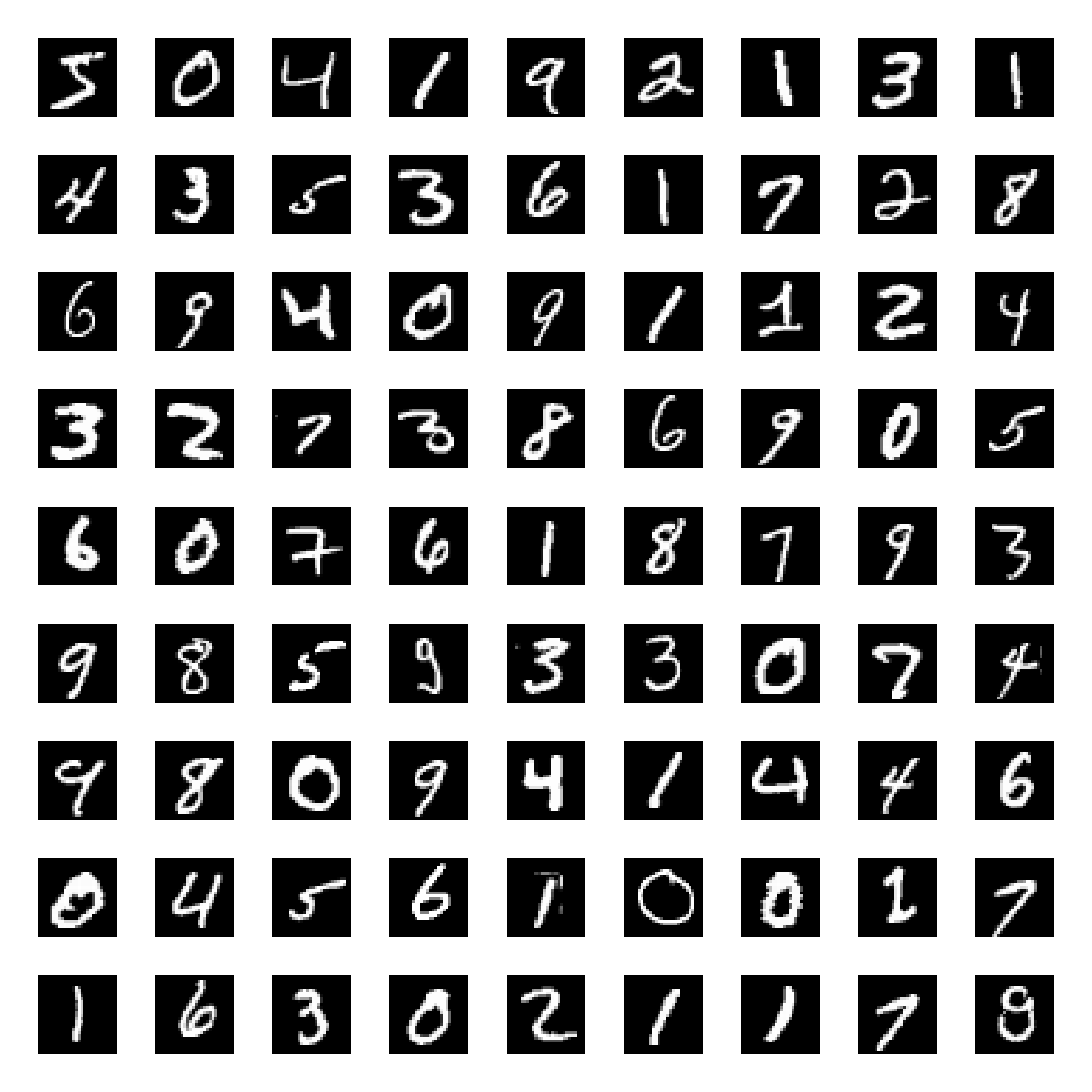Samples from the MNIST datasetꜛ, which is used as input for the nervos SNN in our example below. Each image is 28x28 pixels, which corresponds to 784 input neurons in the network. The pixel intensities are converted to firing frequencies to generate spike trains for the input layer. The network learns to classify these images based on the spiking activity of the output layer neurons.

Input encoding

Each MNIST image is flattened into a vector $p \in [0,1]^{784}$. Pixel intensities are converted to firing frequencies according to

\[f = p \cdot (f_{\max} - f_{\min}) + f_{\min},\]

with typical values $f_{\max} = 70$ Hz and $f_{\min} = 5$ Hz.

For a presentation duration of $T$ discrete simulation steps, each input neuron generates a binary spike train

\[M \in \{0,1\}^{784 \times T},\]

where $M_{ij} = 1$ if neuron $i$ fired at time step $j$.

Thus, the network receives a temporally structured, rate encoded spike pattern.

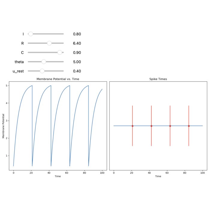
Neuron model: discrete integrate and fire dynamics with adaptive threshold

In practice, nervos does not implement a continuous time leaky integrate and fire differential equation with an explicit leak term. Instead, the neuron state is updated in discrete time steps. For each output neuron $i$ at time step $t$, the membrane potential is incremented by the weighted sum of incoming spikes

\[V_i(t) \leftarrow V_i(t) + \sum_{j=1}^{N_{\text{in}}} w_{ij}\,x_j(t),\]

where $x_j(t)\in{0,1}$ is the presynaptic spike of input neuron $j$ at time step $t$.

After this synaptic integration step, nervos applies a discrete relaxation term whenever the neuron is above its resting potential $V_{\text{rest}}$:

\[\text{if } V_i(t) > V_{\text{rest}}:\; V_i(t)\leftarrow V_i(t) - \Delta_V,\]

with $\Delta_V=\texttt{spike_drop_rate}$. This term plays a stabilizing role similar to a leak, but it is not an exponential decay and it is not derived from a biophysical conductance model.

Each neuron also has a refractory mechanism implemented as a hard time step lock. After a neuron fires or is inhibited at time $t$, it is set to rest until

\[t < t_{\text{rest},i} \equiv t + \tau_{\text{ref}},\]

where $\tau_{\text{ref}}=\texttt{refractory_time}$. While $t < t_{\text{rest},i}$, the neuron does not integrate synaptic input.

The firing threshold is adaptive and implemented as an explicit state variable $\theta_i(t)$, initialized at a baseline value $\theta_0=\texttt{spike_threshold}$. Whenever a neuron fires, its adaptive threshold is increased additively

\[\theta_i(t^+) \leftarrow \theta_i(t) + 1.\]

Additionally, when a neuron is above the resting potential, the adaptive threshold relaxes linearly toward the baseline by a fixed amount per time step

\[\text{if } V_i(t) > V_{\text{rest}} \text{ and } \theta_i(t) > \theta_0:\; \theta_i(t)\leftarrow \theta_i(t) - \Delta_\theta,\]

with $\Delta_\theta=\texttt{threshold_drop_rate}$. Thus, the adaptive threshold dynamics are discrete and piecewise linear rather than exponential with a time constant.

Finally, note that inhibition is implemented as a hard reset of the membrane potential to an inhibitory potential $V_{\text{inh}}=\texttt{inhibitory_potential}$ together with the same refractory lockout. This is a compressed, algorithmic representation of inhibition rather than an explicit inhibitory synapse conductance model.

Synapse models

nervos allows different synapse models, all normalized to

\[w \in [w_{\min}, w_{\max}] = [10^{-3}, 1].\]

Three major models are implemented:

1. Ideal synapse
   Continuous weight updates without quantization.
2. Linear finite state synapse
   Uniform weight steps but with a finite number of discrete states.

3. Nonlinear memristor synapse
   Based on experimental Pr$_{0.7}$Ca$_{0.3}$MnO$_3$ RRAM data. The $i$th weight state of an $n$ state synapse is modeled as

   \[w_i = w_{\max} - \frac{w_{\max} - w_{\min}}{1 - e^{-\nu}} \left[1 - \exp\left(-\nu\left(1 - \frac{i}{n}\right)\right)\right].\]

   The parameter $\nu$ controls the curvature of the nonlinearity.

Initially, all synapses are set to $w = 1$ to facilitate early learning.

STDP learning

Weight changes are driven by an exponential STDP kernel $F(\Delta t)$ with

\[\Delta t = t_{\text{post}} - t_{\text{pre}},\]

and

\[F(\Delta t)= \begin{cases} A_{\text{up}} \exp(-\Delta t/\tau_{\text{up}}), & \Delta t \ge 0,\\ A_{\text{down}} \exp(\Delta t/\tau_{\text{down}}), & \Delta t < 0. \end{cases}\]

Note that nervos also supports alternative STDP kernels such as cosine, sinusoidal, and Gaussian depression-only variants. In the present analysis, however, we focus exclusively on the conventional exponential kernel defined above.

Synaptic updates are applied in a bounded, weight dependent manner. Let $w$ be the current weight and $w_{\min},w_{\max}$ the configured bounds. Define

\[d(w) = \begin{cases} w - w_{\min}, & F(\Delta t) < 0,\\ w_{\max} - w, & F(\Delta t) > 0. \end{cases}\]

Then the update is

\[w \leftarrow w + \eta\,F(\Delta t)\,\text{sign}(d(w))\,|d(w)|^{\gamma},\]

with learning rate $\eta=\texttt{eta}$ and fixed exponent $\gamma=0.9$ in the current implementation. This makes potentiation and depression naturally saturate near the bounds.

STDP is applied only to synapses projecting onto a selected output neuron. In the default Winner Takes All mode (self.wta=True), synaptic updates are applied only for the winner neuron $k(t)$ at each time step where a spike event occurs. This is a strong form of competitive learning.

A further implementation detail is that if no presynaptic spike was observed in the configured past window for a given synapse at that postsynaptic event, nervos still applies a depression update with a randomly chosen negative $\Delta t$ value from a restricted range. This enforces ongoing weakening of synapses that are not consistently supported by correlated pre and post activity, thereby strengthening competition and sparsifying receptive fields.

Training and emergence of classification

During training, each image is presented as an input spike train for $T=\texttt{training_duration}$ discrete time steps. The network is simulated forward, and STDP updates are applied online whenever spiking events occur.

A key point is how nervos constructs the neuron to label association. In the current implementation, the neuron label map is updated online by directly assigning the true label of the current training sample to the neuron that was the maximally excited neuron when the last spike event occurred during that presentation. Denoting this neuron index by $k$, the update is

\[\texttt{neuron_label_map}[k] \leftarrow y,\]

where $y$ is the true class label of the presented sample.

Thus, the label map is not computed via a separate majority vote over winners across the full training set. Instead, it is formed incrementally through repeated overwriting during training, and it stabilizes in practice because neurons that consistently win for a given class will repeatedly reassign themselves to that class.

At test time, classification proceeds without further plasticity. For a test spike train, the network computes winner event counts $c_i$ over the presentation window and returns

\[\hat{y} = \texttt{neuron_label_map}\left[\arg\max_i c_i\right].\]

This readout is algorithmic and relies on the externally stored mapping from neurons to labels. It is therefore best interpreted as a minimal decision rule that extracts class predictions from the emergent winner selective dynamics of the trained output layer.

Synapse bounds and initialization

All synaptic weights are bounded by the configured limits $w_{\min}=\texttt{min_weight}$ and $w_{\max}=\texttt{max_weight}$. In the example configuration used below, these were set explicitly in the parameter dictionary, and the STDP update rule implements saturating weight dependence relative to these bounds.

In the current nervos implementation, the input to output synapse matrix is initialized as

\[W(0)=\mathbf{1},\]

that is all weights start at $w=1$. This choice accelerates early competition and receptive field formation, but it also means that early epochs can show very large weight norms and broad activation patterns before synaptic competition and bounded STDP drive weights toward more selective configurations.

What is stored internally

For detailed analysis, nervos stores (optionally):

• full weight matrix snapshots $W$ after each sample or epoch.
• spike raster matrices for each layer:
  $M^{(\text{layer})}_{\text{epoch}, \text{sample}}$
• learned neuron to label mapping
• synapse state trajectories for finite state models

From $W$, we can, e.g., compute receptive fields by reshaping

\[w_i \in \mathbb{R}^{784}\]

into $28 \times 28$ images, directly visualizing digit templates emerging in single neurons.

From spike rasters, we can compute:

• winner indices
• spike statistics
• L1 and L2 norms of synaptic vectors
• weight evolution curves

Thus, the framework allows a full dynamical and structural analysis of learning.

What nervos’ SNN does and does not achieve

While nervos is in my view a powerful tool to study STDP and synapse models, it is important to understand its strengths and limitations in the context of computational neuroscience and neuromorphic engineering.

Strengths

The main strengths of the nervos SNN are:

• fully local learning rule without global error backpropagation
• hardware aware synapse models including memristor nonlinearity
• very small architecture
• good performance under small training sets
• transparent internal dynamics

In small five class MNIST tasks, the authors report over 90% accuracy with conventional STDP and ideal synapses. When extended to all ten classes, accuracy drops to around 76%, which is still impressive for such a minimal architecture and purely local learning rule.

Limitations

The main limitations of the nervos SNN are:

• Two layer architecture only.
• Rate based input encoding, not true temporal coding.
• No deep hierarchical feature extraction.
• Classification relies on post hoc label assignment: It relies on an external label map that is built during training by repeatedly assigning the current sample label to the winning neuron, and is then used at test time to map the $\arg\max$ spike count neuron to a class label.
• Accuracy drops significantly when synapse states are strongly quantized.

Compared to fully biological plausible cortical microcircuits, the network is extremely simplified:

• no dendritic compartmentalization,
• no recurrent excitatory loops,
• no neuromodulation, and
• no reward signals.

Nevertheless, it provides a clean minimal platform to study STDP and hardware constraints.

Python example: Pattern Recognition on MNIST

Before we begin and for reproducibility, here is the environment setup that I have used for this example:

conda create -n nervos python=3.12 mamba -y
conda activate nervos
mamba install -y numpy matplotlib ipykernel requests
pip install nervos

I used nervos version 0.0.5, which is the latest version at the time of writing. The code is structured in a way that should be compatible with future versions, but some adjustments may be needed if the API changes significantly.

So, let’s start with the imports and some global settings for plotting:

import os
import numpy as np
import matplotlib.pyplot as plt
import nervos as nv

# set global properties for all plots:
plt.rcParams.update({'font.size': 12})
plt.rcParams["axes.spines.top"]    = False
plt.rcParams["axes.spines.bottom"] = False
plt.rcParams["axes.spines.left"]   = False
plt.rcParams["axes.spines.right"]  = False

Parameter setup

First, we define the parameters for the simulation. We will use 500 images of the MNIST training set for training and 150 images of the test set for testing. The training duration is set to 100 discrete time steps, which is sufficient for the network to process the input and generate spikes. We also set various parameters related to the neuron and synapse models, as well as the learning rates for STDP. We can also choose the number of classes we want to train on, e.g., 5 (MNIST subset) or 10 (full MNIST set). In this example, we will use 6 classes (digits 0 to 5) to keep the training time manageable while still demonstrating the learning capabilities of the network.

All parameters are stored in a Parameters object from the nervos library, which allows for easy access and modification throughout the code:

RESULTS_PATH = "figures"
os.makedirs(RESULTS_PATH, exist_ok=True)

# choose classes here:
CLASSES = list(range(6))   # choose any value between 1 and 10
identifier_name = f"{len(CLASSES)}classmnist"

p = nv.Parameters()

parameters_dict = {
    "training_images_amount": 500, # nervos is very memory hungry especially when m.get_spikeplots = True and m.get_weight_evolution = True (!); either use smaller numbers here, or set those to False below, or run it on a machine with high RAM
    "testing_images_amount": 150,
    "training_duration": 100, # discrete simulation time units
    "past_window": -10,
    "epochs": 3,  # note: after each epoch, the training set is not reshuffled, so the same images are presented in the same order.
    "image_size": [28, 28],
    "resting_potential": -70,
    "input_layer_size": 784,
    "output_layer_size": 80,
    "inhibitory_potential": -100,
    "spike_threshold": -55,
    "reset_potential": -90,
    "spike_drop_rate": 0.8,
    "threshold_drop_rate": 0.4,
    "min_weight": 1e-05,
    "max_weight": 1.0,
    "A_up": 0.8,
    "A_down": -0.3,
    "tau_up": 5,
    "tau_down": 5,
    "eta": 0.03,
    "min_frequency": 1,
    "max_frequency": 50,
    "refractory_time": 15,
    "tau_m": 10,
    "conductance": 10
}
for key, value in parameters_dict.items():
    setattr(p, key, value)

Note, that nervos is very memory hungry especially when m.get_spikeplots = True and m.get_weight_evolution = True (see below). Either use smaller numbers for the training and testing images (like ~500 and ~150, respectively), or set those settings to False, or run it on a machine with enough RAM.

Helper functions and class definitions

Next, we set up some functions which we need for the implementation of the MNIST_SNN class and for the analysis of the results.

We begin with the MNIST_SNN class which is a wrapper around the nervos SNN that handles data loading, training, and prediction. We also add a method to plot random samples from the dataset, which will be useful for visualizing the input spike trains before training the model. The plot_random_samples method takes care of aggregating the spike trains over time to reconstruct the original images for visualization, since the MNIST images are not stored as pixel values but only as spike trains in the model:

class MNIST_SNN(nv.Module):
    def __init__(self, parameters, identifier=None, classes=None, train_size=None, test_size=None, seed=None):
        super().__init__(parameters, identifier)

        # set default (5) if not provided
        if classes is None:
            classes = list(range(5))
        self.classes = list(classes)

        self.dataloader = nv.dataloader.MNISTLoader(parameters, classes=self.classes)

        # if you want the loader sizes to be controllable from outside:
        if train_size is None:
            train_size = getattr(parameters, "training_images_amount", 100)
        if test_size is None:
            test_size = getattr(parameters, "testing_images_amount", 20)

        self.X_train, self.Y_train = self.dataloader.dataloader(
            preprocess=True, pca=False, size=int(train_size), seed=seed)
        self.X_test, self.Y_test = self.dataloader.dataloader(
            preprocess=True, train=False, pca=False, size=int(test_size), seed=seed)

    def predict(self, un_processed_image, model_location):
        spike_train = np.array(self.dataloader.img2spiketrain(un_processed_image))
        synapses, neuron_label_map = self.load_model(model_location)
        return self.get_prediction(spike_train, synapses, neuron_label_map)

    def plot_random_samples(self, N=10, train=True, aggregate="sum", seed=None, cmap="hot_r", figsize=(10, 10)):
        """
        Plot N random MNIST samples from train or test set.

        Parameters
        ----------
        N : int
            Number of samples to plot.
        train : bool
            If True: use training set, else test set.
        aggregate : str
            "sum" or "mean" over time to reconstruct image from spike train.
        seed : int or None
            Optional seed for reproducibility.
            
            
        Note:
        -----
        nervos' dataloader directly returns spike trains for the MNIST images, 
        which we can visualize here before training the model. This also means,
        the MNIST images are not stored as pixel values in the model, but only 
        as spike trains. We therefore need to aggregate the spike trains over 
        time to reconstruct the original image for visualization.
        """

        if seed is not None:
            np.random.seed(seed)

        X = self.X_train if train else self.X_test
        Y = self.Y_train if train else self.Y_test

        indices = np.random.choice(len(X), size=min(N, len(X)), replace=False)

        cols = min(N, 5)
        rows = int(np.ceil(N / cols))

        plt.figure(figsize=figsize)

        for i, idx in enumerate(indices):
            spike_train = X[idx]  # shape: (784, T)

            if aggregate == "sum":
                img_vec = spike_train.sum(axis=1)
            elif aggregate == "mean":
                img_vec = spike_train.mean(axis=1)
            else:
                raise ValueError("aggregate must be 'sum' or 'mean'")

            img = img_vec.reshape(28, 28)

            plt.subplot(rows, cols, i + 1)
            plt.imshow(img, cmap=cmap, interpolation="nearest")
            plt.title(f"Label: {Y[idx]}")
            plt.axis("off")

        plt.tight_layout()

The next function is a direct replication of the original visualize_synapse function from the nervos tutorial, which visualizes the learned synaptic weights for each class. It aggregates the synaptic weights of all neurons that are assigned to the same class and reshapes them into 28x28 images to visualize the receptive fields learned by the network for each digit class:

def visualize_synapse(synapses, labels, cmap="hot_r", figsize=(10, 30), ncols=5):
    kk = 28
    labels = np.asarray(labels)

    classes = {i: np.zeros((kk, kk)) for i in np.unique(labels)}
    for idx in range(len(synapses)):
        classes[labels[idx]] += synapses[idx].reshape((kk, kk))

    class_keys = sorted(classes.keys())
    n_classes = len(class_keys)
    ncols = max(1, int(ncols))
    nrows = int(np.ceil(n_classes / ncols))

    plt.figure(figsize=figsize)
    for i, k in enumerate(class_keys, start=1):
        plt.subplot(nrows, ncols, i)
        plt.imshow(classes[k], cmap=cmap, interpolation="nearest")
        plt.title(f"{k}")
        plt.axis("off")

    plt.tight_layout()

To evaluate the performance of the model, we need to compute the accuracy on the test set. We use again a provided function from the nervos tutorial, called accuracy, which takes the trained model and the test classes as input, generates spike trains for the test images, and computes the predicted labels based on the output layer activity. It then compares the predicted labels to the true labels to calculate the overall accuracy of the model:

def accuracy(m2, classes, parameters_dict):
    loader = nv.dataloader.MNISTLoader(m2.parameters, classes=list(classes))
    spike_trains, labels = loader.dataloader(train=False, preprocess=True, 
      seed=123, size=parameters_dict["testing_images_amount"])

    t = 0
    c = 0
    preds = []
    print("Calculating Accuracy")
    for st, label in zip(spike_trains, labels):
        pred = m2.get_prediction(st)
        preds.append(pred)
        c += int(pred == label)
        t += 1
        print(f"\rTested {t} images", end="")
    print()
    print(c / t)
    return labels, preds

For a more detailed analysis of the model’s performance, we can compute the confusion matrix, which shows how many times each true class was predicted as each possible class. The following function confusion_matrix_np computes the confusion matrix which is used in the plot_confusion_matrix function to visualize it. The confusion matrix can be normalized to show percentages instead of raw counts, which can be helpful for interpretation:

def confusion_matrix_np(y_true, y_pred, labels):
    """
    Calculate the confusion matrix.
    Rows: true labels
    Cols: predicted labels
    """
    y_true = np.asarray(y_true, dtype=int)
    y_pred = np.asarray(y_pred, dtype=int)
    labels = np.asarray(labels, dtype=int)

    k = labels.size
    idx = {lab: i for i, lab in enumerate(labels)}
    C = np.zeros((k, k), dtype=int)

    for t, p in zip(y_true, y_pred):
        if (t in idx) and (p in idx):
            C[idx[t], idx[p]] += 1
    return C

def plot_confusion_matrix(C, labels, normalize=False, title=None, cmap="Greys"):
    """
    Plot confusion matrix. If normalize=True: row-normalize 
    (per true label).
    """
    C = np.asarray(C)
    if normalize:
        row_sums = C.sum(axis=1, keepdims=True).astype(float)
        row_sums[row_sums == 0.0] = 1.0
        M = C / row_sums
    else:
        M = C

    fig, ax = plt.subplots(figsize=(6, 5))
    im = ax.imshow(M, interpolation="nearest", cmap=cmap)
    cbar = fig.colorbar(im, ax=ax, fraction=0.046, pad=0.04)

    ax.set(
        xticks=np.arange(len(labels)),
        yticks=np.arange(len(labels)),
        xticklabels=[str(x) for x in labels],
        yticklabels=[str(x) for x in labels],
        xlabel="Predicted Labels",
        ylabel="True Labels",
        title=title if title is not None else ("Confusion matrix (normalized)" if normalize else "Confusion matrix"))

    # annotate:
    fmt = ".2f" if normalize else "d"
    thresh = M.max() * 0.6 if M.size else 0.0
    for i in range(M.shape[0]):
        for j in range(M.shape[1]):
            ax.text(
                j, i, format(M[i, j], fmt),
                ha="center", va="center",
                color="white" if M[i, j] > thresh else "black")

    plt.tight_layout()
    return fig, ax

The next function actually repeats the accuracy function but uses the confusion matrix to compute the overall accuracy. It takes the confusion matrix as input and calculates the accuracy as the trace (sum of diagonal elements) divided by the total number of samples. It also computes the recall for each class, which is the diagonal element divided by the sum of the corresponding row (true positives / total actual positives):

def accuracy_metrics(C):
    """
    From confusion matrix C (rows=true, cols=pred):
    accuracy.
    """
    C = np.asarray(C, dtype=float)
    total = C.sum()
    acc = np.trace(C) / total if total > 0 else np.nan

    row_sums = C.sum(axis=1)
    with np.errstate(divide="ignore", invalid="ignore"):
        recall = np.diag(C) / row_sums

    return acc, recall

An important aspect of analyzing the model’s performance is to look at the spike trains of the output neurons. The following rasterplot function creates a raster plot for the binary spike matrix, where each dot represents a spike from a neuron at a specific time step. The function also allows highlighting specific neurons (e.g., the epoch winner and the final winner) with different colors and sizes to visually distinguish them from the rest of the neurons:

def rasterplot(
    spike_train: np.ndarray,
    title: str = "raster",
    xlim=None,
    highlight_neuron_idx: int | None = None,
    highlight_color: str = "orange",
    highlight2_neuron_idx: int | None = None,
    highlight2_color: str = "magenta",
    base_color: str = "0.35",
    s_base: float = 2.0,
    s_highlight: float = 8.0,
    s_highlight2: float = 8.0):
    """
    Raster plot for a binary spike matrix with up to two highlighted neurons.

    spike_train: shape (N, T), entries 0/1
    highlight_neuron_idx: epoch wise winner (orange)
    highlight2_neuron_idx: final winner (magenta, retroactive)
    If both indices are equal, only one overlay is drawn (orange), but the legend
    label indicates "epoch winner = final winner".
    """
    spike_train = np.asarray(spike_train)
    if spike_train.ndim != 2:
        raise ValueError(f"spike_train must be 2D (N,T), got shape {spike_train.shape}")

    N, T = spike_train.shape
    ys, xs = np.where(spike_train == 1)

    plt.figure(figsize=(10, 4))
    plt.scatter(xs, ys, s=s_base, color=base_color, linewidths=0)

    handles = []

    def _overlay(idx: int, color: str, size: float, label: str):
        if not (0 <= idx < N):
            raise ValueError(f"highlight idx={idx} out of bounds for N={N}")
        xs_h = np.where(spike_train[idx] == 1)[0]
        if xs_h.size == 0:
            return None
        ys_h = np.full(xs_h.shape, idx, dtype=int)
        return plt.scatter(xs_h, ys_h, s=size, color=color, linewidths=0, label=label)

    j1 = int(highlight_neuron_idx) if highlight_neuron_idx is not None else None
    j2 = int(highlight2_neuron_idx) if highlight2_neuron_idx is not None else None
    same = (j1 is not None) and (j2 is not None) and (j1 == j2)

    # epoch winner (always, if provided)
    if j1 is not None:
        label1 = f"epoch winner = final winner idx {j1}" if same else f"epoch winner idx {j1}"
        h1 = _overlay(j1, highlight_color, s_highlight, label1)
        if h1 is not None:
            handles.append(h1)

    # final winner (only if provided and different)
    if (j2 is not None) and (not same):
        h2 = _overlay(j2, highlight2_color, s_highlight2, f"final winner idx {j2}")
        if h2 is not None:
            handles.append(h2)

    if handles:
        plt.legend(loc="best")

    if xlim is not None:
        plt.xlim(xlim)

    plt.xlabel("time step")
    plt.ylabel("neuron index")
    plt.grid(True, axis="x", linestyle="--", alpha=0.6)
    plt.title(title)
    plt.tight_layout()

To visualize the receptive fields of the output neurons, we define the following function plot_rf_of_neuron, which takes the synaptic weights of the first layer and a specific neuron index as input. It reshapes the weight vector of that neuron into a 28x28 image and visualizes it using a colormap. This allows us to see what kind of input pattern that neuron has learned to respond to:

def plot_rf_of_neuron(
    synapses_0: np.ndarray,
    neuron_idx: int,
    title: str = "",
    cmap: str = "viridis",
    figsize=(3.0, 3.0)) -> None:
    """
    Plot receptive field (weights reshaped to 28x28) of one output neuron.

    synapses_0: shape (n_out, 784)
    """
    w = np.asarray(synapses_0)[neuron_idx]  # (784,)
    img = w.reshape(28, 28)

    plt.figure(figsize=figsize)
    plt.imshow(img, cmap=cmap, interpolation="nearest")
    plt.title(title)
    plt.axis("off")
    plt.tight_layout()

The function plot_label_template visualizes a class specific weight template derived from the trained network. It selects all output neurons whose entry in neuron_label_map equals the given label and then averages their input weight vectors (or sums them, depending on mode). The resulting 784 dimensional vector is reshaped to 28×28 and plotted. This is therefore not an average MNIST image, but an average of learned synaptic weight patterns for that class. We use this function to visualize the emergent digit templates learned by the network for each class, which can be compared to individual receptive fields of single winner neurons as well as to the aggregated input spike representations of real MNIST samples, in order to assess how closely the learned synaptic structure aligns with the underlying data distribution:

def plot_label_template(
    synapses_0: np.ndarray,
    neuron_label_map: np.ndarray,
    label: int,
    title: str = "",
    cmap: str = "viridis",
    mode: str = "sum",  # "sum" or "mean"
    figsize=(3.0, 3.0)) -> None:
    """
    Plot label template: aggregate RFs of all neurons assigned to a given label.
    """
    synapses_0 = np.asarray(synapses_0)
    nlm = np.asarray(neuron_label_map)

    idx = np.where(nlm == int(label))[0]
    plt.figure(figsize=figsize)

    """ 
    idx.size indicates how many neurons are mapped to this label. 
    If idx.size == 0, it means no neuron is mapped to this label.
    """

    if idx.size == 0:
        plt.text(0.5, 0.5, f"No neurons mapped to label {label}", ha="center", va="center")
        plt.axis("off")
        plt.title(title)
        plt.tight_layout()
        return

    W = synapses_0[idx]  # (n_label_neurons, 784)
    if mode == "sum":
        img = W.sum(axis=0).reshape(28, 28)
    elif mode == "mean":
        img = W.mean(axis=0).reshape(28, 28)
    else:
        raise ValueError("mode must be 'sum' or 'mean'")

    plt.imshow(img, cmap=cmap, interpolation="nearest")
    plt.title(title + f" (neurons mapping: {idx.size}/{synapses_0.shape[0]})")
    plt.axis("off")
    plt.tight_layout()

The next functions are utility functions to extract the winner neuron index based on spike counts and to get the last weight snapshot for a specific sample and epoch. These functions will be useful for analyzing the evolution of the winner neuron’s receptive field over epochs:

def get_winner_neuron_idx(m, epoch, train_image_idx):
    spk_out = np.asarray(m.spikeplots[epoch][train_image_idx][-1])  # (n_out, T)
    spike_counts = spk_out.sum(axis=1)
    return int(np.argmax(spike_counts)), spike_counts

def get_last_weight_snapshot_for_sample(m, epoch, train_image_idx):
    """
    weight_evolution[epoch][sample] is a list of snapshots.
    Each snapshot has shape (n_out, n_in).
    """
    snapshots = m.weight_evolution[epoch][train_image_idx]
    if snapshots is None or len(snapshots) == 0:
        raise ValueError("No weight evolution stored. Set m.get_weight_evolution=True before training.")
    return np.asarray(snapshots[-1])  # (n_out, n_in)

def plot_winner_rf_evolution_over_epochs(
    m,
    train_image_idx,
    last_epoch=None,
    cmap="viridis",
    parameters_dict=None,
    nlm_final=None,):
    """
    For each epoch, pick the winner neuron by spike count
    (same definition as in your raster loop), then plot its RF from the
    epoch specific weight snapshot and compute summary metrics for that same winner.

    Notes:
      - The "winner" can change across epochs (that is the point).
      - If nlm_final is given, we also show map=... in the titles (final neuron label map).
    """
    if last_epoch is None:
        last_epoch = m.parameters.epochs - 1

    true_label = int(m.Y_train[train_image_idx])

    rfs = []
    norms_l1 = []
    norms_l2 = []
    means = []

    winner_idxs = []
    winner_counts = []
    winner_maps = []

    for ep in range(m.parameters.epochs):
        # epoch specific winner from spikes (same as your raster loop)
        spk_out = np.asarray(m.spikeplots[ep][train_image_idx][-1])  # (n_out, T)
        spike_counts = spk_out.sum(axis=1)
        winner_idx = int(np.argmax(spike_counts))
        winner_count = int(spike_counts[winner_idx])

        winner_map = None
        if nlm_final is not None and winner_idx < len(nlm_final):
            winner_map = int(nlm_final[winner_idx])

        # epoch specific weights (last snapshot for this sample at this epoch)
        W = get_last_weight_snapshot_for_sample(m, ep, train_image_idx)  # (n_out, 784)
        w = W[winner_idx]  # (784,)

        if w.size != 28 * 28:
            raise ValueError(
                f"Expected 784 weights for RF, got {w.size}. W shape is {W.shape}.")

        rfs.append(w.reshape(28, 28))
        norms_l1.append(np.sum(np.abs(w)))
        norms_l2.append(np.sqrt(np.sum(w**2)))
        means.append(np.mean(w))

        winner_idxs.append(winner_idx)
        winner_counts.append(winner_count)
        winner_maps.append(winner_map)

    # RF tiles
    n = len(rfs)
    fig, axes = plt.subplots(1, n, figsize=(3 * n, 3), squeeze=False)
    for ep in range(n):
        ax = axes[0, ep]
        ax.imshow(rfs[ep], cmap=cmap, interpolation="nearest")

        if winner_maps[ep] is None:
            ax.set_title(f"Epoch {ep}\nidx={winner_idxs[ep]}, spikes={winner_counts[ep]}")
        else:
            ax.set_title(
                f"Epoch {ep}\nidx={winner_idxs[ep]}, spikes={winner_counts[ep]}, map={winner_maps[ep]}"
            )

        ax.axis("off")

    plt.suptitle(
        f"Winner RF evolution for sample {train_image_idx}\ntrue={true_label}")
    plt.tight_layout()
    plt.savefig(os.path.join(RESULTS_PATH, f"winner_rf_evolution_sample{train_image_idx}_tiles.png"),dpi=200)
    plt.close()


    # summary metrics:
    fig, ax1 = plt.subplots(figsize=(6, 4))

    l1_line, = ax1.plot(norms_l1, marker="o", label="L1 norm")
    l2_line, = ax1.plot(norms_l2, marker="o", label="L2 norm")

    ax1.set_xlabel("Epoch")
    ax1.set_ylabel("L1 / L2 value")
    ax1.set_title(f"Weight summary for epoch wise winners (sample {train_image_idx})")
    # annotate eg at the L2 dots, which winner idx they correspond to:
    for ep in range(n):
        # ax1.annotate(f"winner\nidx {winner_idxs[ep]}", (ep, norms_l2[ep]), 
        #              textcoords="offset points", xytext=(0,10), ha='center', fontsize=8)
        ax1.annotate(f"winner\nidx: {winner_idxs[ep]}", (ep, np.max(norms_l1)*1.1), 
                     textcoords="offset points", xytext=(0,10), ha='center', fontsize=10,
                     va="top")
    ax1.set_ylim(bottom=0, top=np.max(norms_l1)*1.2)

    # secondary axis for mean weight:
    ax2 = ax1.twinx()
    mean_line, = ax2.plot(means, marker="o", linestyle="--", color="gray", label="Mean weight")
    ax2.set_ylabel("Mean weight", color="gray")
    ax2.tick_params(axis="y", labelcolor="gray")

    if parameters_dict is not None:
        ax2.set_ylim(bottom=parameters_dict["min_weight"], top=parameters_dict["max_weight"])
    else:
        ax2.set_ylim(bottom=0, top=1.01)

    # unified legend
    lines = [l1_line, l2_line, mean_line]
    labels = [line.get_label() for line in lines]
    ax1.legend(lines, labels, loc="best")
    plt.tight_layout()
    plt.savefig(os.path.join(RESULTS_PATH, f"winner_rf_evolution_sample{train_image_idx}_summary.png"), dpi=200)
    plt.close()

Loading data and training the model

Having defined all the necessary classes and functions, we can now proceed to load the data. We use nervos’ own dataloader.MNISTLoader to load the MNIST dataset and initialize the layers of the SNN. We also plot some random samples from the training and test sets to visualize the input spike trains before training the model:

m = MNIST_SNN(p, identifier_name, classes=CLASSES)
m.initialise_layers([784,80])

m.plot_random_samples(N=25, train=True, aggregate="sum", seed=42, cmap="viridis", figsize=(8,9))
plt.suptitle("Random samples from the training set (aggregated over time (sum))")
plt.tight_layout()
plt.savefig(os.path.join(RESULTS_PATH, "random_samples_train.png"), dpi=200)
plt.close()
m.plot_random_samples(N=25, train=False, aggregate="sum", cmap="viridis", figsize=(8,9))
plt.suptitle("Random samples from the test set (aggregated over time (sum))")
plt.tight_layout()
plt.savefig(os.path.join(RESULTS_PATH, "random_samples_test.png"), dpi=200)
plt.close()

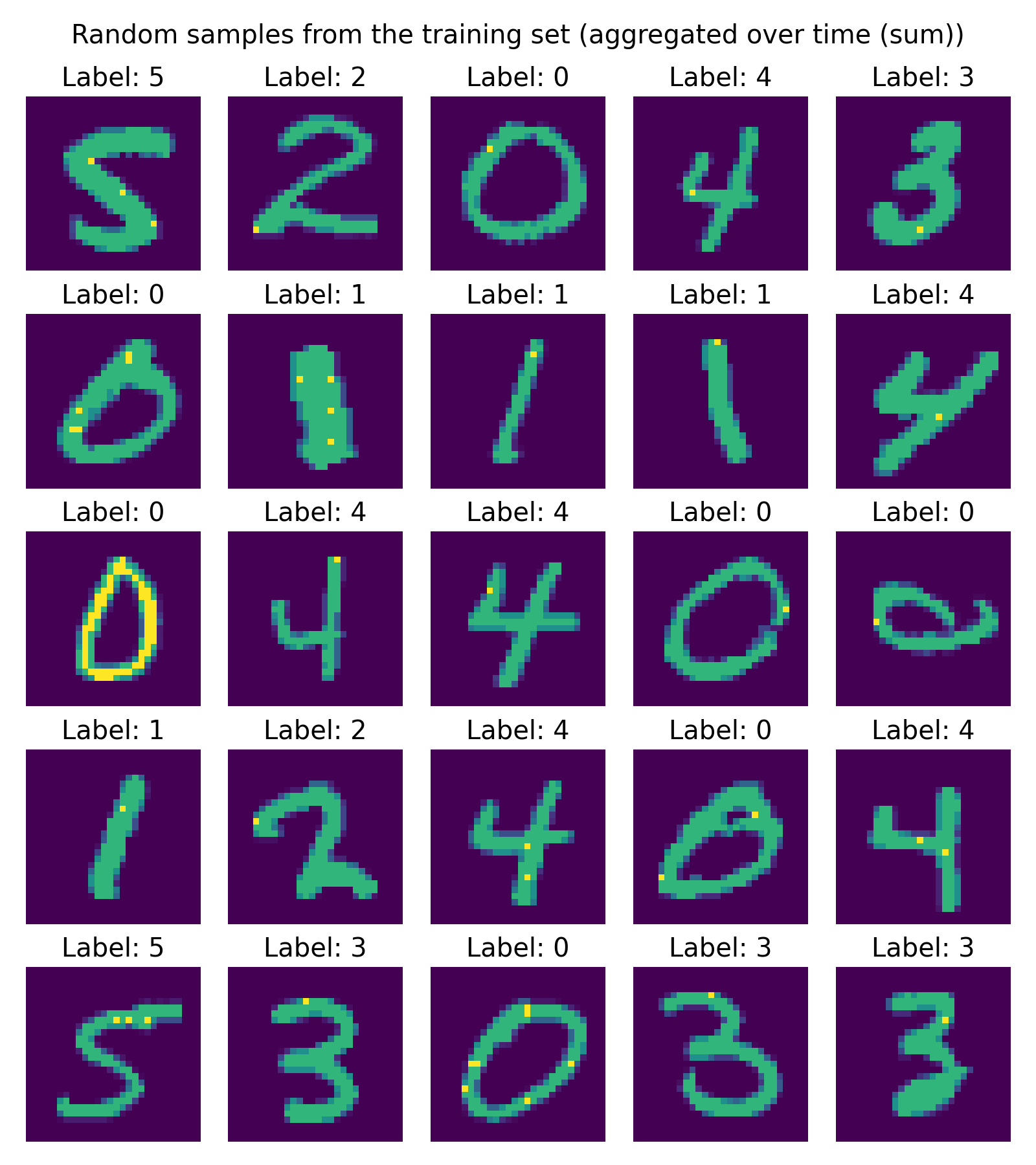Samples from the training set, visualized by aggregating the input spike trains over time (sum) to reconstruct the original images. Each image is labeled with its true class. This gives us an intuition of what kind of input patterns the network will be trained on.

Finally, we run the training loop of the model and evaluate its performance. The training loop will save the learned synapses and neuron label map at the end of each epoch in a subdirectory named “Epoch_{epoch_number}-{accuracy}” for easy identification of the best epoch later on:

m.get_spikeplots = True
m.get_weight_evolution = True
y = m.train()

In the next section, we will analyze the results of the training by visualizing the learned synapses and evaluating the accuracy of the model on the test set.

Evaluation

The first evaluation step is to visualize the learned synapses. We aggregate synaptic weight vectors across output neurons that share the same label in the learned neuron_label_map, and visualize the resulting class conditioned templates as 28x28 images. This allows us to see what kind of input patterns the network has learned to associate with each digit class:

# evaluate the model by visualizing the learned synapses and calculating accuracy on test set:
visualize_synapse(m.learned_synapses[0], m.learned_neuron_label_map, figsize=(8, 5.0), cmap="viridis")
plt.suptitle("Learned synapses\n(summed over output neurons of the same predicted class)")
plt.tight_layout()
plt.savefig(os.path.join(RESULTS_PATH, "learned_synapses.png"), dpi=200)
plt.close()

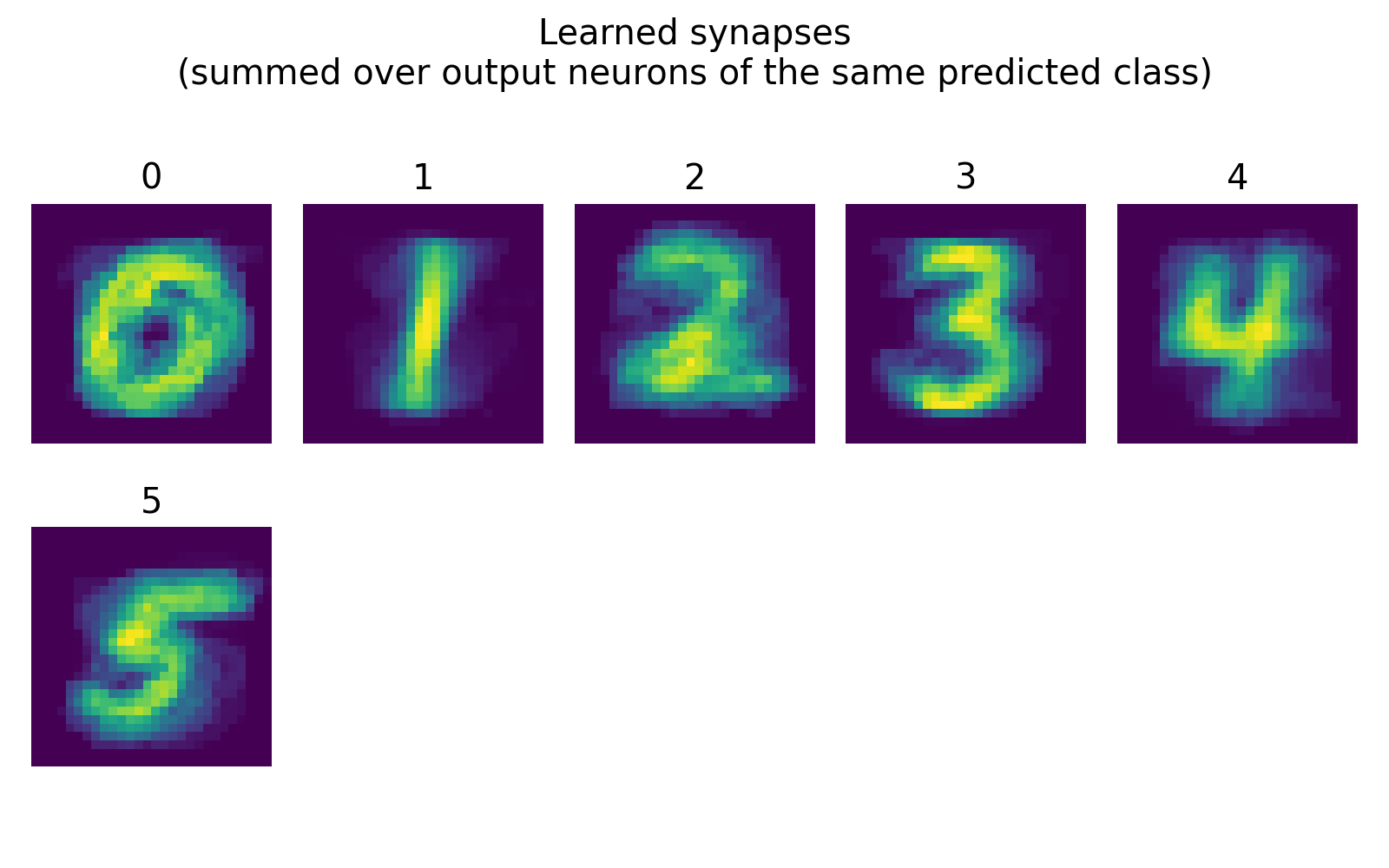Learned synapses, visualized by summing over output neurons of the same predicted class. We trained the model on the classes 0 to 5, and we can see that the learned synaptic patterns for each class show distinct features that resemble the corresponding digit shapes, indicating that the network has successfully learned to differentiate between the classes based on the input spike patterns.

In our case, we can see that the learned synapses for each class show distinct patterns that resemble the corresponding digit shapes, indicating that the network has successfully learned to differentiate between the classes based on the input spike patterns.

Accuracy evaluation on test set

Next, we evaluate the accuracy of the model on the test set. We use the accuracy function to get the true and predicted labels for the test samples, then compute the confusion matrix and overall accuracy metrics. Finally, we plot the confusion matrix both in raw counts and normalized form to visualize how well the model is performing across different classes:

# evaluate accuracy on test set:
y_true,y_pred = accuracy(m, classes=CLASSES, parameters_dict=parameters_dict)

# calculate confusion matrix and metrics:
labels = CLASSES  # use the selected classes
C = confusion_matrix_np(y_true, y_pred, labels=labels)
acc, recall = accuracy_metrics(C)
print("Accuracy:", acc)
print("Recall:", recall)
# plot confusion matrix:
plot_confusion_matrix(C, labels=labels, normalize=False, title="Confusion matrix (counts)",cmap="Blues")
plt.savefig(os.path.join(RESULTS_PATH, "confusion_matrix_counts.png"), dpi=200)
plt.close()
plot_confusion_matrix(C, labels=labels, normalize=True, title="Confusion matrix (row-normalized)", cmap="Blues")
plt.savefig(os.path.join(RESULTS_PATH, "confusion_matrix_normalized.png"), dpi=200)
plt.close()

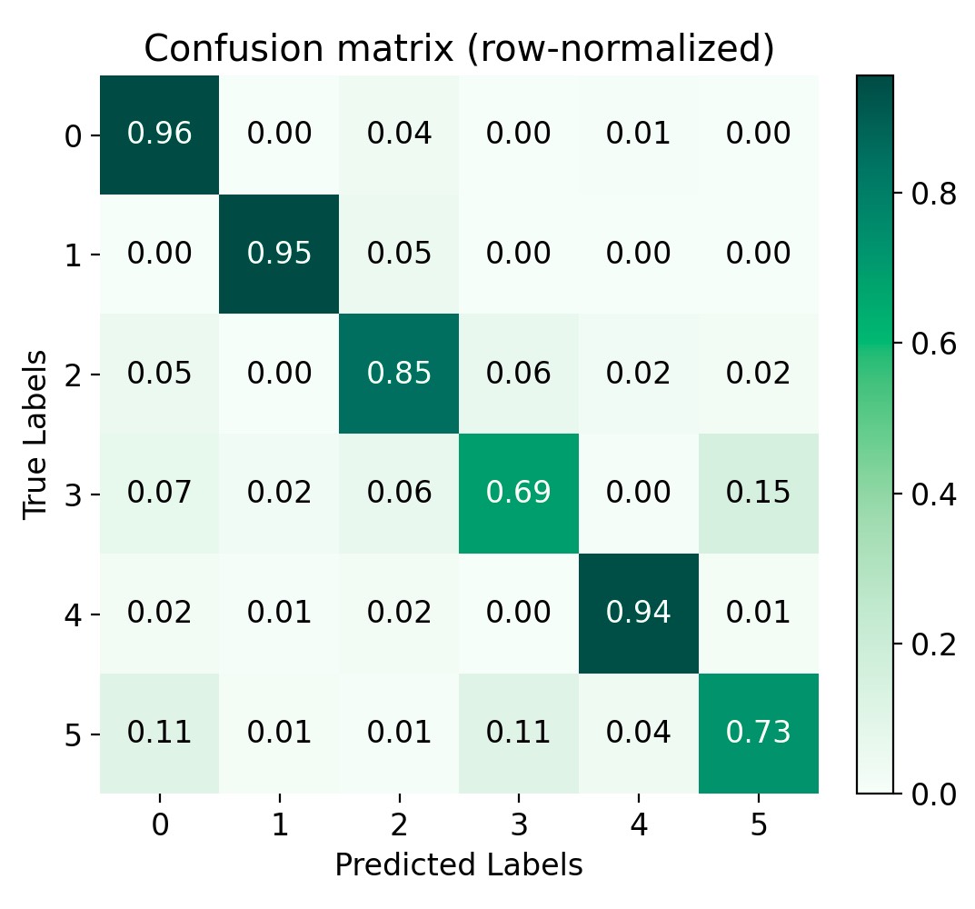Confusion matrix, row-normalized. This allows us to see how well the model is performing across different classes.

With our model and training parameters defined above, we reach an accuracy of around 0.85 on the test set, which is already quite good. The confusion matrix also indicated that almost all classes are well recognized, i.e., most of the predictions are on the diagonal, with only a few misclassifications. This suggests that the model has successfully learned to differentiate between the digit classes based on the input spike patterns.

Spike activity and winner neuron RF evolution

Next, we will take a closer look at the spike activity of the output neurons and the evolution of the winner neuron’s receptive field over epochs for specific training samples. We will visualize the spike raster plots for the output layer at each epoch and also plot the receptive fields of the winner neurons to see how they evolve during training and how they relate to the learned synaptic weights and the true labels of the samples:

# spike rasterplots and winner RF evolution for specific training samples:
train_image_idx_list = [41, 61]
synapses_final = m.learned_synapses[0]
nlm_final      = m.learned_neuron_label_map
for train_image_idx in train_image_idx_list:
    true_label = int(m.Y_train[train_image_idx])
    final_epoch = p.epochs - 1
    final_winner_idx, _ = get_winner_neuron_idx(m, final_epoch, train_image_idx)
    for epoch in range(p.epochs):
        
        # pick winner from spikes (epoch-specific)
        spk_in  = m.spikeplots[epoch][train_image_idx][0]    # epoch, sample/train image, layer (0: Input, 1: Output)
        spk_out = m.spikeplots[epoch][train_image_idx][-1] 
        spike_counts = spk_out.sum(axis=1)
        winner_idx   = int(np.argmax(spike_counts))
        winner_count = int(spike_counts[winner_idx])
        
        # spike raster plot for the output layer at this epoch and this training image:
        rasterplot(spk_out,
            title=(f"Output raster, epoch {epoch} sample {train_image_idx} "
                   f"(true={true_label}, current winner={winner_idx}, final winner={final_winner_idx})"),
            xlim=(0, spk_out.shape[1]),
            highlight_neuron_idx=winner_idx,
            highlight_color="orange",
            highlight2_neuron_idx=final_winner_idx,
            highlight2_color="magenta")
        plt.savefig(os.path.join(RESULTS_PATH, f"raster_output_neurons_epoch{epoch}_sample{train_image_idx}.png"), dpi=200)
        plt.close()

        # predicted label according to the (final) neuron_label_map:
        winner_label = int(nlm_final[winner_idx]) if winner_idx < len(nlm_final) else -1

        
        # epoch specific weights:
        W_ep = get_last_weight_snapshot_for_sample(m, epoch, train_image_idx)

        # 1. RF of the CURRENT epoch winner (this is what you want additionally):
        winner_label = int(nlm_final[winner_idx]) if winner_idx < len(nlm_final) else -1
        plot_rf_of_neuron(
            W_ep,
            winner_idx,
            title=(
                f"Epoch winner RF in epoch {epoch}\n on sample {train_image_idx}: neuron idx={winner_idx},\n"
                f"spikes={winner_count}, map={winner_label}, true={true_label}"),
            cmap="viridis",
            figsize=(3.8, 4.0))
        plt.savefig(os.path.join(RESULTS_PATH, f"rf_epochWinner_epoch{epoch}_sample{train_image_idx}.png"), dpi=200)
        plt.close()

        # 2. RF of the FINAL winner, but using CURRENT epoch weights (optional, if you also want this):
        final_label = int(nlm_final[final_winner_idx]) if final_winner_idx < len(nlm_final) else -1
        final_count_this_epoch = int(spike_counts[final_winner_idx])
        plot_rf_of_neuron(
            W_ep,
            final_winner_idx,
            title=(
                f"Final winner RF in epoch {epoch}\n on sample {train_image_idx}: neuron idx={final_winner_idx},\n"
                f"spikes(ep)={final_count_this_epoch}, map={final_label}, true={true_label}"),
            cmap="viridis",
            figsize=(3.8, 4.0))
        plt.savefig(os.path.join(RESULTS_PATH, f"rf_finalWinner_asOfEpoch{epoch}_sample{train_image_idx}.png"), dpi=200)
        plt.close()
        
        # now plot the label template:
        plot_label_template(
            synapses_final,
            nlm_final,
            true_label,
            title=f"Template sample {train_image_idx} in epoch {epoch}:\ntrue={true_label}",
            cmap="viridis",
            mode="mean",
            figsize=(3.8, 4.0))
        plt.savefig(os.path.join(RESULTS_PATH, f"rf_template_epoch{epoch}_sample{train_image_idx}.png"), dpi=200)
        plt.close()

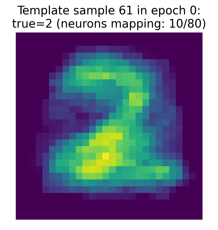
The template for the true label of the sample, which has been learned by the network as an aggregate of the synaptic weights of all output neurons that are mapped to that label. This template gives an intuition of the prototypical input pattern that the network has learned to associate with that class (here: the digit “2”), and can be compared to the RF of the winner neuron and to the original input image to see how closely they align.

Epoch 0

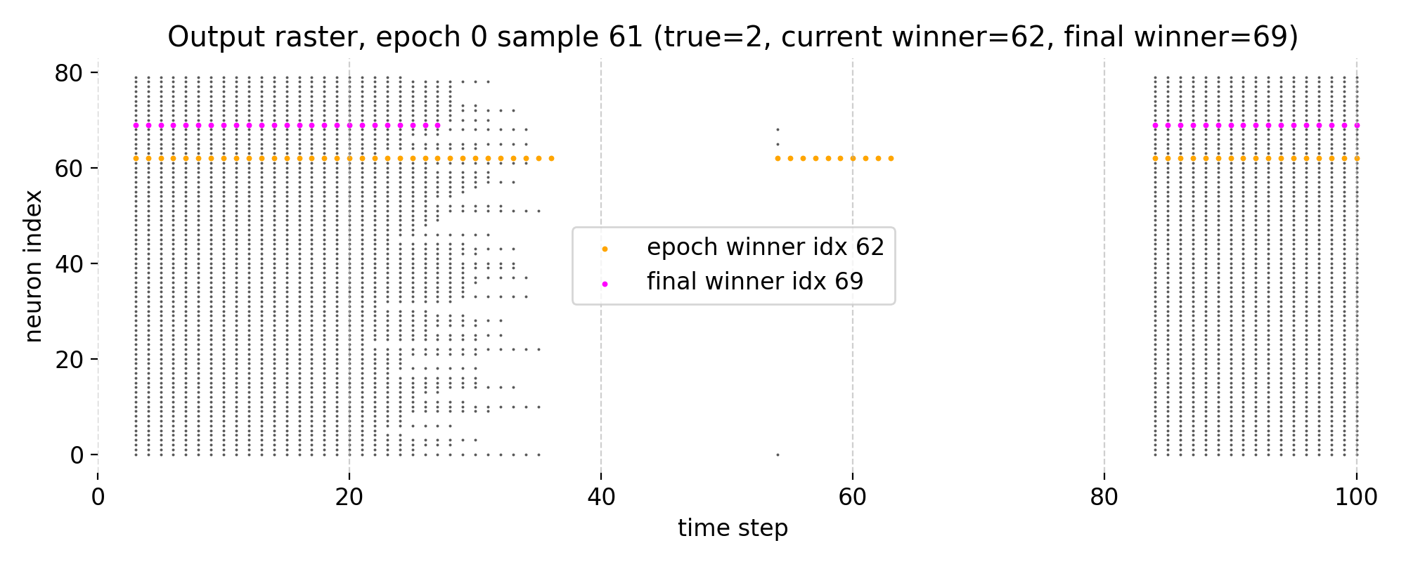
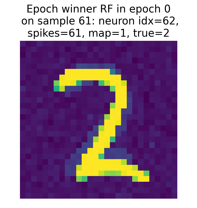
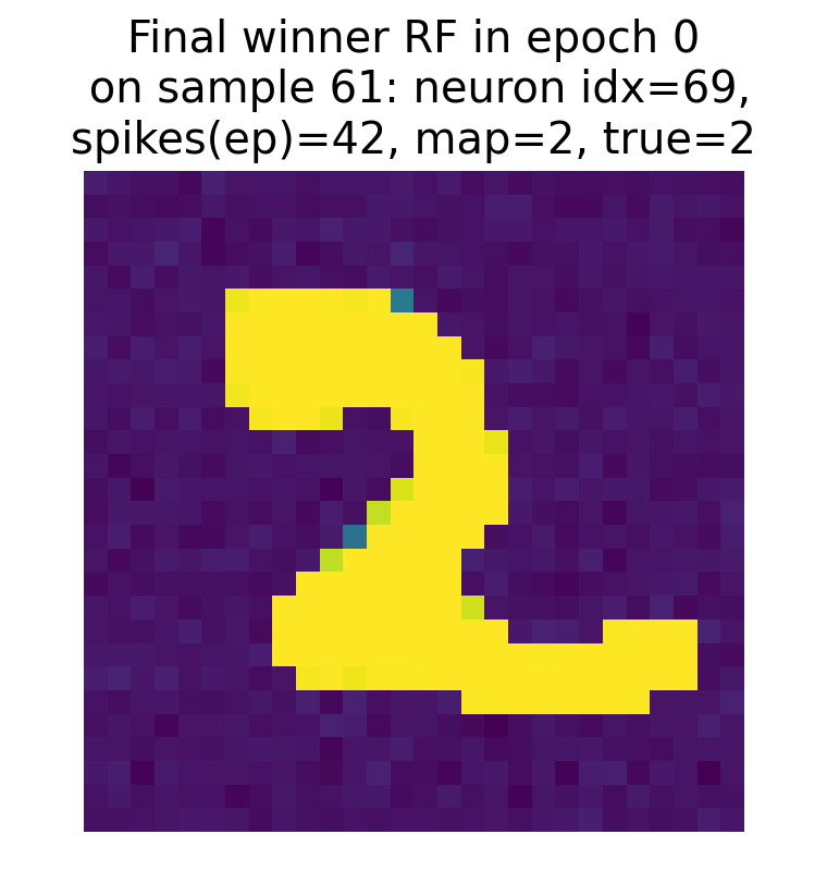
Top: Raster plot of output neuron activity in epoch 0 for sample 61. Each dot represents a spike from a neuron at a specific time step. The highlighted neurons indicate the epoch winner (orange) and the final winner (magenta; i.e., the neuron that wins in the final epoch 3). Bottom left: Receptive field of the winner neuron in epoch 0 for sample 61, visualized as a 28x28 image of its synaptic weights. Bottom right: Receptive field of the final winner neuron as of epoch 0 for sample 61, visualized using the same weights but highlighting the final winner neuron.

The raster plot shows the spiking activity of the output layer neurons over time for a single training image at epoch 0. Here, we have 80 output neurons (as defined in the parameters) and the x-axis represents the discrete time steps of the simulation (100 + 1). Each dot in the raster plot corresponds to a spike from a particular neuron at a specific time step. The plot shows an initial firing during the ongoing exposure to the input image, followed by a damping of activity due to adaptation or inhibition. The pattern of spiking depends on the learned synaptic weights and the input. Later, we reach threshold and the output neurons fire again, which can be seen as a second wave of spiking. This behavior is overall controlled by

• the refractory time,
• the spike drop rate, and
• the adaptive threshold.

The timing and pattern of these spikes are crucial for the model’s predictions and learning process.

Note that nervos uses two related but not identical notions of a “winner”: during training, the label map is updated using the neuron with the highest membrane potential at the spike event (specifically the last such event in the presentation), whereas in our analysis we define the winner as the neuron with maximal spike count over the full presentation window.

However, as implemented in nervos, this is not a biologically detailed simulation with biophysically plausible temporal dynamics as we have

• no synaptic delays,
• no continuous integration of membrane potential over time (instead, the potential is updated in discrete time steps based on incoming spikes and current synaptic weights),
• no real membrane potential dynamics/ODE (like leaky integration, conductance-based synapses, etc.), and
• no real WTA (winner-takes-all) inhibition between output neurons. Inhibition is implemented algorithmically: At each spike event, neurons that do not exceed threshold are forced to an inhibitory potential and placed in refractory lockout, rather than receiving explicit inhibitory synaptic conductances.

However, the discrete time steps and the spike patterns still allow us to analyze the learning dynamics and the evolution of the synaptic weights in a way that is analogous to how we would analyze a more biologically detailed SNN, albeit with some caveats regarding the interpretation of the membrane potential traces and spike timings.

The two bottom plots show the receptive fields of the winner neuron in epoch 0 and the final winner neuron as of epoch 0, respectively. The RF is visualized as a 28x28 image of the synaptic weights from the input layer to that specific output neuron. The RF of the winner neuron in epoch 0 already shows the structure that resembles the input pattern “2”. However, the mapped label of that neuron shows “1”, which indicates that at this early stage of training, the neuron has not yet learned to correctly associate its RF with the true label of the sample.

The RF of the final winner neuron as of epoch 0 also shows a similar pattern, but it is important to note that the final winner neuron can change across epochs, and its RF will evolve during training as the synaptic weights are updated based on the STDP learning rule. However, already in this first epoch 0, it maps to the correct label “2”, which suggests that it has already started to learn the correct association, even though its RF is not yet fully developed.

Epoch 1

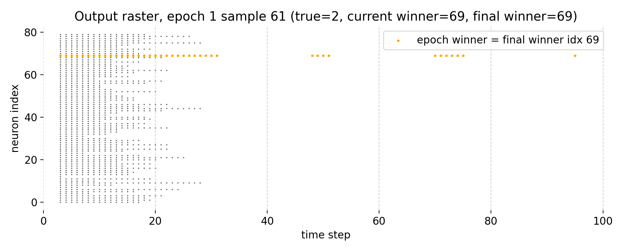
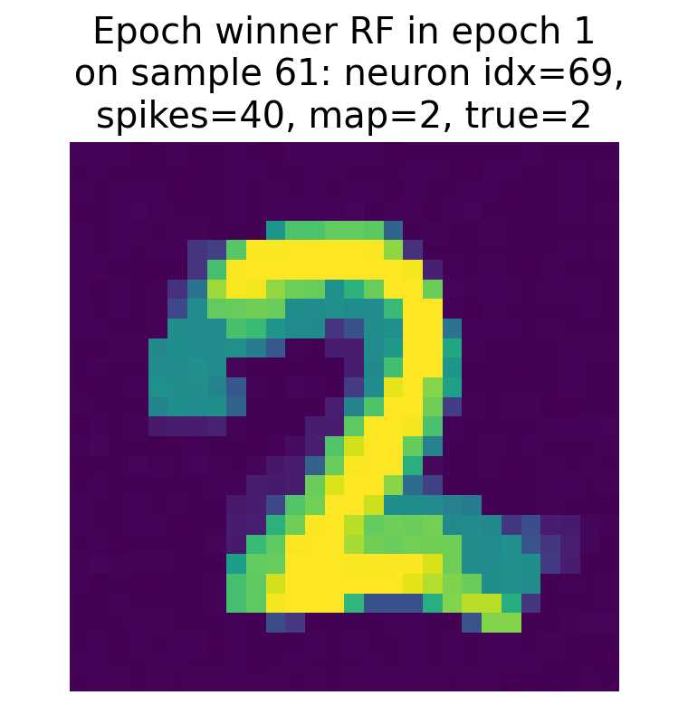
Top: Raster plot of output neuron activity in epoch 1 for sample 61. Bottom left: Receptive field of the winner neuron in epoch 1 for sample 61. Bottom right: Receptive field of the final winner neuron as of epoch 1 for sample 61. Note, that in this epoch, the current winner neuron and the final winner neuron are the same.

In epoch 1, the winner neuron changes from index 62 to index 69, which is the index of the final winner neuron at the end of the training. Thus, the final neuron already dominates the spike activity during this training sample, reflecting a stabilization of the network’s internal representation for this sample.

The raster plot on the other hand shows a reduction in overall spiking activity compared to epoch 0, indicating increased selectivity and stronger competition among output neurons.

Epoch 2

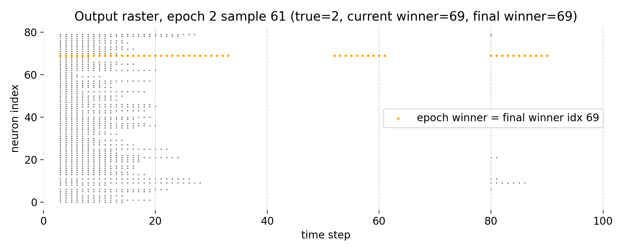
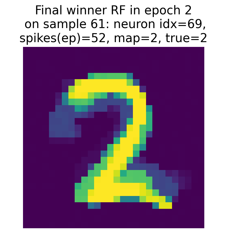
Top: Raster plot of output neuron activity in epoch 2 for sample 61. Bottom left: Receptive field of the winner neuron in epoch 2 for sample 61. Bottom right: Receptive field of the final winner neuron as of epoch 2 for sample 61. Note, that in this final epoch, the current winner neuron and the final winner neuron are the same.

In the final epoch 2, neuron 69 remains the winner and now consistently dominates the spike activity. The predicted label matches the true label, demonstrating successful specialization of this neuron for the digit “2”. The receptive field of this neuron 69 also appears more broadened, indicating that STDP has reinforced synaptic weights from a wider range of input pixels that are relevant for recognizing the digit, which is a sign of successful learning and generalization.

The raster plot shows a further refinement of activity, with reduced distributed firing across other neurons. This suggests that the network has converged toward a more selective representation for this digit.

Weight evolution of the winner neuron

Finally, we can also plot the evolution of the synaptic weights of the winner neuron across epochs to see how its receptive field develops during training. This will allow us to see how the synaptic weights are updated based on the STDP learning rule and how they converge to a stable pattern that corresponds to the learned representation for that sample:

# let's plot the evolution of the synaptic weights over epochs for the winner neuron of the last epoch:
for train_image_idx in train_image_idx_list:
    plot_winner_rf_evolution_over_epochs(m, train_image_idx=train_image_idx, cmap="viridis",
                                         parameters_dict=parameters_dict, nlm_final=nlm_final)

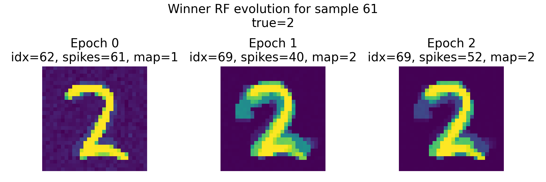
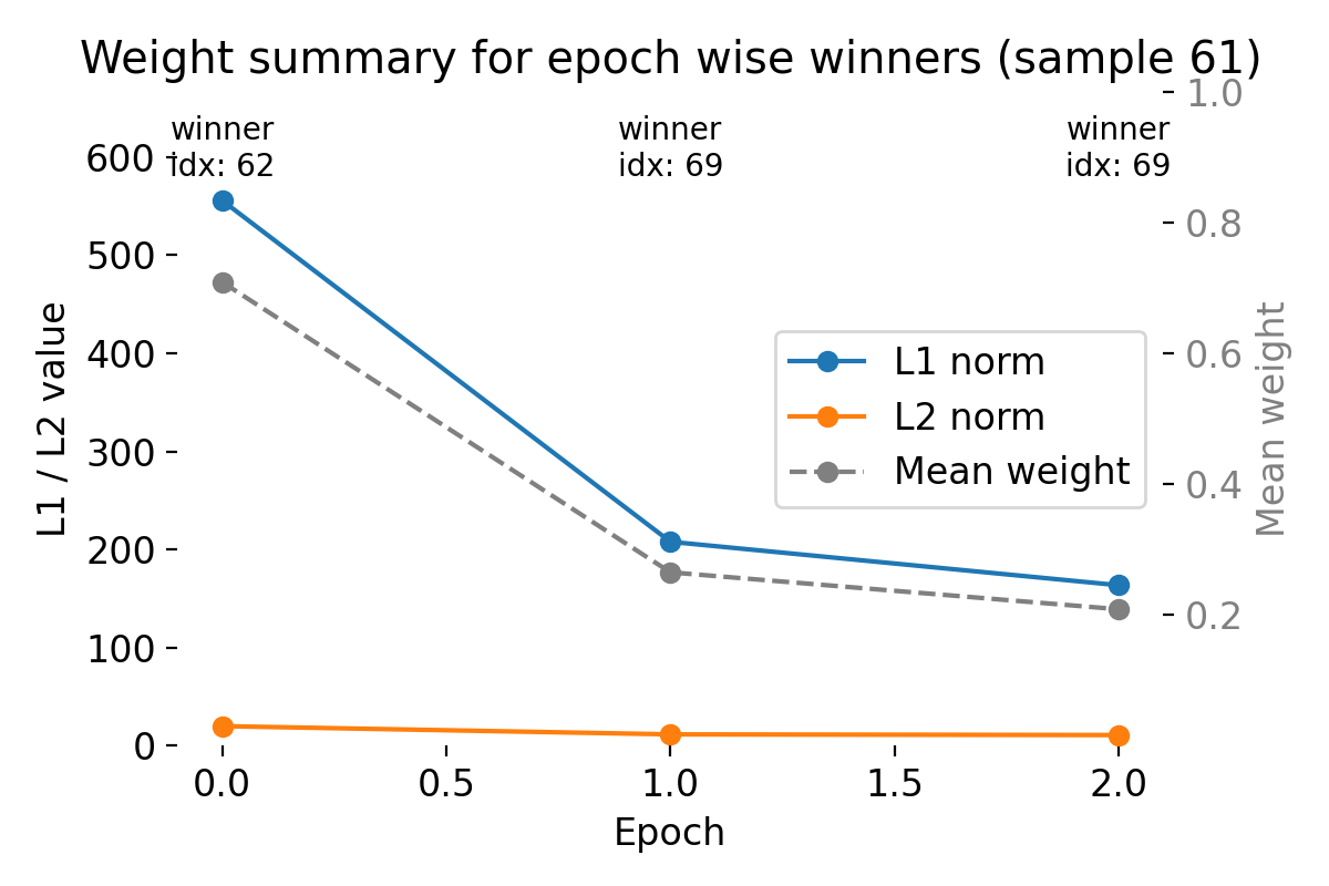Top: Evolution of the receptive field of the winner neuron across epochs for sample 61, visualized as tiles. Each tile shows the RF of the winner neuron at a specific epoch, allowing us to see how it evolves during training. The title of each tile indicates the epoch number, the index of the winner neuron, its spike count, its mapped label according to the final neuron label map, and the true label of the sample. Bottom: Summary plot of weight metrics (L1 norm, L2 norm, and mean weight) for the winner neurons across epochs for sample 61.

The top panel shows the receptive field of the epoch-wise winner neuron for sample 61 across training epochs. Importantly, the winner neuron is defined separately in each epoch as the neuron with the highest spike count for this specific input sample. Consequently, the identity of the winner can change between epochs.

In epoch 0, neuron 62 wins with 61 spikes and is mapped to label 1 according to the final neuron label map. Its receptive field already resembles the digit “2” in structure, but the class association is still incorrect. We have recognized this already in the previous section. The weight pattern is relatively diffuse, and the L1 and L2 norms are comparatively large, indicating a broadly distributed weight configuration.

In epoch 1, the winner switches to neuron 69. This neuron is mapped to label 2 and therefore aligns with the true class of the sample. The receptive field still resembles the digit “2”, but is now a bit more “smeared out”, which is not a bad thing, as it indicates that the neuron is integrating information from a broader set of input pixels that are relevant for recognizing the digit. The spike count of this winner neuron is 40, which is slightly lower than the previous winner. The weight norms decrease substantially compared to epoch 0. This reflects a redistribution and normalization of synaptic weights under the STDP dynamics and weight constraints.

In epoch 2, neuron 69 remains the winner. The receptive field changes only moderately compared to epoch 1, suggesting stabilization of the learned representation. The weight norms decrease slightly further, while the overall shape remains consistent. This indicates convergence toward a stable attractor-like weight configuration for this sample.

The bottom summary plot quantifies this evolution:

• The L1 norm decreases strongly from epoch 0 to epoch 1 and slightly further to epoch 2.
• The L2 norm shows a similar but less pronounced decline.
• The mean weight also decreases across epochs.

This reduction does not imply loss of information. Instead, it reflects synaptic competition and bounded, weight dependent saturation inherent to the implemented STDP update, together with the adaptive threshold dynamics. Early in training, weights are more broadly distributed. As learning progresses, weights become more selective and concentrated on input pixels that consistently co activate with the winner neuron.

Crucially, because the winner neuron can change across epochs, the summary metrics track the weights of different neurons at different times. This is intentional: the plot characterizes the weight profile of whichever neuron currently dominates the representation of this sample (compare the raster plots above), rather than following a single fixed neuron.

Overall, the combined RF tiles and norm curves illustrate three key aspects of learning in nervos:

1. Early competition between output neurons for representing a pattern.
2. Reassignment of dominance to a neuron whose label mapping matches the true class.
3. Gradual stabilization and sharpening of the receptive field under repeated exposure.

This provides a transparent view of how discrete-time STDP, adaptive thresholds, and weight constraints together drive the formation of class-specific receptive fields in the output layer.

Conclusion

In my view, nervos provides a deliberately minimal, transparent framework for studying how local spike timing dependent plasticity interacts with synapse models that range from ideal floating point weights to hardware constrained finite state and nonlinear memristor inspired devices. The core appeal is that essentially every relevant mechanism remains inspectable: Input encoding, spike generation, winner selection, weight updates, and the emergence of neuron selectivity can be analyzed directly from stored spike rasters and weight snapshots, without any implicit gradient based optimization.

In this post, we closely followed nervos’ official MNIST tutorialꜛ and extended it with additional analyses of internal dynamics. Using a two layer network with 784 input neurons and 80 output neurons, and using only local STDP weight updates, the model reached an accuracy of roughly 85% on a six class test set. The learned synapse visualizations and the class specific weight templates indicated that the network develops digit like weight patterns, consistent with the idea that the output population self organizes into feature selective units.

The winner based analyses highlight how this self organization plays out on single samples. For the inspected training example with true label “2”, the epoch wise winner changed from one output neuron to another between early and later epochs. The receptive fields showed an interpretable progression from an initial pattern with an incorrect final label mapping, toward a stable winner neuron whose mapping matched the true class. Tracking weight norms across epochs showed a strong reduction in L1 and L2 magnitudes when the winner switched, consistent with competitive redistribution under STDP together with weight clipping and the adaptive threshold dynamics. In other words, the network does not merely accumulate weights monotonically. It reallocates representational dominance across output neurons until repeated wins make the label assignment stable in practice, because the same neuron is repeatedly reassigned to the same class.

At the same time, it is also important to be explicit about what kind of model this is and is not. nervos captures a few key computational motifs that are often discussed in theoretical accounts of unsupervised cortical learning: local plasticity, competition, and specialization of units. However, it is not a biologically detailed simulator of spiking circuits. The time axis is discrete, the neuronal dynamics are simplified relative to continuous conductance based models, the inhibition is implemented in a simplified global inhibition scheme, and there is no anatomical or physiological structure beyond a fully connected feedforward projection with global competition. Most importantly, classification is not implemented by an intrinsic downstream readout population but by a post hoc interpretation step, namely the neuron label map constructed online by repeatedly assigning the current sample label to the winning neuron and then applied to $\arg\max$ spike counts. This is a legitimate algorithmic readout, but it is not the same as a biological circuit that must produce a decision through spikes alone.

These points also clarify where nervos sits relative to biologically plausible architectures. Compared to models that aim for cortical realism, such as recurrent networks with structured excitation and inhibition, synaptic delays, dendritic nonlinearities, and neuromodulatory or reward gated learning, nervos is far simpler and leaves out many mechanisms that matter for real neural computation. Those richer models can express temporal codes, recurrent memory, context dependence, and credit assignment mechanisms beyond local STDP. They also often avoid the need for an explicit label map by embedding a readout circuit into the model itself. The cost is that they become harder to analyze and harder to link to neuromorphic constraints in a clean way. And, also an important point, they often require more computational resources to simulate, which can limit the scope of systematic parameter sweeps and mechanistic analyses.

Overall, Maskeen and Lashkare did a fantastic job! I think the main strengths of nervos are conceptual clarity, transparence, and practical accessibility. The minimal architecture makes it easy to attribute observed behavior to specific design choices, and the framework is explicitly designed to compare learning rules and synapse implementations under controlled conditions. This is valuable both for neuromorphic engineering, where non ideal synapses are the rule rather than the exception, and for computational neuroscience, where it can serve as a clean baseline for what purely local plasticity and competition can achieve on a pattern recognition problem.

If you are interested in exploring the code and running the simulations yourself, I highly recommend checking out the official nervos GitHub repositoryꜛ and read the according pre-printꜛ.

The complete code used in this blog post is available in this Github repositoryꜛ (nervos_snn_mnist.py). Feel free to modify and expand upon it, and share your insights.

References and further reading

• Maskeen, Jaskirat Singh; Lashkare, Sandip, A Unified Platform to Evaluate STDP Learning Rule and Synapse Model using Pattern Recognition in a Spiking Neural Network, 2025, arXiv:2506.19377, DOI: 10.48550/arXiv.2506.19377ꜛ
• Maskeen, Jaskirat Singh; Lashkare, Sandip, A Unified Platform to Evaluate STDP Learning Rule and Synapse Model using Pattern Recognition in a Spiking Neural Network, ICANN 2025, Springerꜛ
• nervos GitHub repositoryꜛ
• nervos documentationꜛ
• LeCun, Yann; Bottou, Léon; Bengio, Yoshua; Haffner, Patrick, Gradient-based learning applied to document recognition, 1998, Proceedings of the IEEE, doi: 10.1109/5.726791ꜛ
• Diehl, Peter U.; Cook, Matthew, Unsupervised learning of digit recognition using spike-timing-dependent plasticity, 2015, Frontiers in Computational Neuroscience, doi: 10.3389/fncom.2015.00099ꜛ
• N. Caporale, & Y. Dan, Spike timing-dependent plasticity: a Hebbian learning rule, 2008, Annu Rev Neurosci, Vol. 31, pages 25-46, doi: 10.1146/annurev.neuro.31.060407.125639ꜛ
• G. Bi, M. Poo, Synaptic modifications in cultured hippocampal neurons: dependence on spike timing, synaptic strength, and postsynaptic cell type, 1998, Journal of neuroscience, doi: 10.1523/JNEUROSCI.18-24-10464.1998ꜛ
• Wulfram Gerstner, Werner M. Kistler, Richard Naud, and Liam Paninski, Chapter 19 Synaptic Plasticity and Learning in Neuronal Dynamics: From Single Neurons to Networks and Models of Cognition, 2014, Cambridge University Press, ISBN: 978-1-107-06083-8, free online versionꜛ
• Robert C. Malenka, Mark F. Bear, LTP and LTD, 2004, Neuron, Vol. 44, Issue 1, pages 5-21, doi: 10.1016/j.neuron.2004.09.012
• Nicoll, A Brief History of Long-Term Potentiation, 2017, Neuron, Vol. 93, Issue 2, pages 281-290, doi: 10.1016/j.neuron.2016.12.015ꜛ
• Jesper Sjöström, Wulfram Gerstner, Spike-timing dependent plasticity, 2010, Scholarpedia, 5(2):1362, doi: 10.4249/scholarpedia.1362ꜛ