LaTeX Guide
\(\LaTeX\) is a typesetting software developed for mathematical writing and widespread in academia. It comes with its own markup language ꜛ, which allows easy typesetting of mathematic expressions. \(\LaTeX\) enables the user to focus purely on the writing of content, while text formatting and the correct placement of graphics and tables are automatically performed by predefined settings. Even the table of contents as well as the bibliography, list of figures and tables are created effortlessly.
\LaTeX markup.
In this guide, we will cover the basics of writing a document with \(\LaTeX\), including the correct representation of mathematical expressions, text formatting, and the creation of tables and figures. We will also cover how to create a bibliography and how to cross-reference within your document. All together enabling you to create a well-structured and visually appealing document with ease, which you can directly apply to your next scientific paper, thesis, or report.
Default LaTeX document
A default \(\LaTeX\) document looks as follows:
\documentclass[14pt]{article}
% This part is the preamble of your document

\begin{document}
% This part reserved for your content

\end{document}
Explanations:
| Document part | Description |
|---|---|
| documentclass | Defines the type of your document. The most common classes are article, report and book, or scrartcl, scrrprt and scrbook. You can also add extra options like letterpaper or a4paper to set the document format, twocolumn to use a two columns layout, or twoside for automatically setting the margins for a two-sided document.Within the square brackets you define the default font size of your document. |
| preamble | Here you define all required document settings that overwrite or extend the default settings. Also, here you can include extra packages that might be required for special markups within your document. This is also the place for defining variables for later usage within your document. |
| document | This part is reserved for your actual content. |
% |
Initiates a comment. |
The format in which your document will be saved is a .tex file. The output file generated after the compilation of your .tex file is a PDF or PS (PostScript) file.
Correct representation of mathematical expressions
It is important, that mathematical expressions and pure text are visually distinguishable within a document. Therefore, mathematical functions, equations and variables are always displayed in italics (e.g., \(x=9\), \(f(x)=x^2\pi^{-1}\)). This rule does not account for predefined functions, e.g., the sine or cosine function (\(\sin(x)\), \(\cos(x)\)), and physical units. With \(\LaTeX\), you can easily represent mathematical expressions in a correct way.
Title page
To define an optional title page – or header, depending on the chosen document class – simply add the following markups to the preamble as well as the \maketitle command at the beginning of the document section:
\documentclass[12pt]{article}

\title{My document's title}
\date{2021}
\author{Jane Doe}

\begin{document}
\maketitle

Lorem ipsum dolor sit amet, consectetur adipiscing elit. Fusce et erat eget mauris semper aliquam in non nulla. Quisque a velit semper, varius lacus at, egestas ante. Morbi aliquam viverra elit eu volutpat.

\end{document}

Text formatting
| Command | Rendered Text |
|---|---|
This is \textbf{bold}. |
This is $\textbf{bold}$. |
This is \textit{italicized}. |
This is $\textit{italicized}$. |
This is \underline{underlined}. |
This is $\underline{underlined}$. |
This is \emph{emphasized}. |
This is $\textit{emphasized}$. |
This is \texttt{typewriter family}. |
This is $\texttt{typewriter family}$. |
This is \textrm{Roman font family}. |
This is $\textrm{Roman font family}$. |
This is \textsf{sans serif font}. |
This is $\textsf{sans serif font}$. |
You can also assign an enclosed environment for the text formattings shown above:
| Enclosed environment | Rendered Text |
|---|---|
{\bfseries This is bold.} |
$\textbf {This is bold.}$ |
{\itshape This is italicized.} |
$\textit{This is italicized.}$ |
{\em This is emphasized.} |
$\textit{This is emphasized.}$ |
{\ttfamily This is typewriter family.} |
$\texttt{This is typewriter family.}$ |
{\rmfamily This is bold.} |
$\textrm {This is Roman font family.}$ |
{\sffamily This is bold.} |
$\textsf {This is sans serif font.}$ |
Normal text in math mode: If you want to display text in math mode, use the \text{your text} command (e.g., $ x=10 \text{while} y=7$ renders to $x=10\; \text{while}\; y=7$ instead of $x=10\; while\; y=7$ without the \text command).
Boldface in math mode: The math mode can contain boldface by using the \mathbf{your text} command (e.g., $\mathbf{R}$ renders to $\mathbf{R}$).
Blackboard bold in math mode: The math mode can contain blackboard bold by using the \mathbb{your text} command (e.g., $\mathbb{R}$ renders to $\mathbb{R}$). \mathbb can be used to express the set of natural numbers ($\mathbb{N}$), integers ($\mathbb{Z}$), rational numbers ($\mathbb{Q}$), real numbers ($\mathbb{R}$), or complex numbers ($\mathbb{C}$).
Undefined control sequence…: If you receive a warning like “Undefined control sequence…” either when you try to use $\mathbb{...}$ or $\mathbf{...}$, please include the amssymb as well as the amsmath package in your preamble (\usepackage{amssymb}, \usepackage{amsmath}).
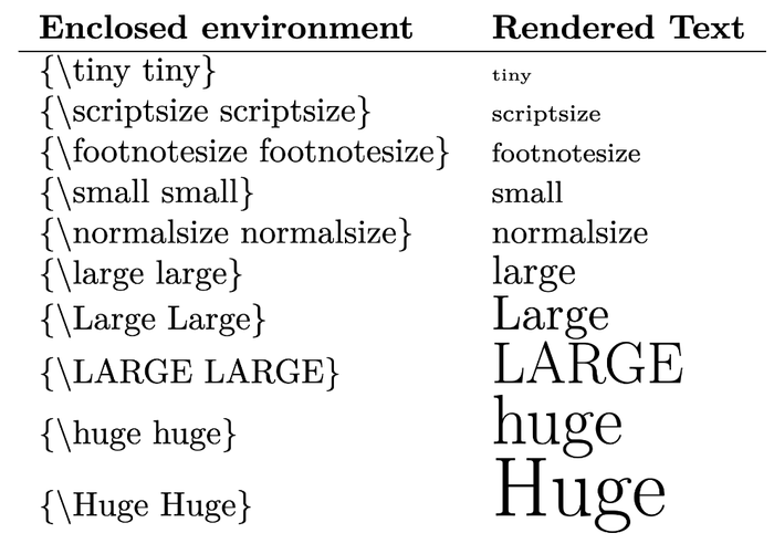
Font size
Font color
You need to include the xcolor package in your preamble (\usepackage{xcolor}). Then, within your document use the \textcolor{color}{your text} command, e.g.,
This is \textcolor{red}{my text in \textbf{red}}.
This is my text in red.
You can use one of the following predefined colors: white, gray, black, red, green, blue, cyan, magenta, or yellow. Or define your own colors in the preamble:
\usepackage{xcolor}
\definecolor{my_blue}{RGB}{0, 115, 207}
...
This is  \textcolor{my_blue}{my color}.
Online color pickers: You can use online HTML color pickers like htmlcolorcodes.com ꜛ to find the RGB values of your desired color.
Headings
| Available headings |
|---|
\part{Title of a part} |
\chapter{Title of a chapter} |
\section{Title of a section} |
\subsection{Title of a sub-section} |
\subsubsection{Title of a sub-sub-section} |
\paragraph{Title of a paragraph} |
\subparagraph{Title of a sub-paragraph} |
Suppress heading numbering: Adding an asterisks * right after the heading command (e.g., \chapter*{Title of a chapter}) suppresses both, the numbering of the heading as well as its entry in the table of contents.
\part and \chapter are only available in the document classes book and report.
Text alignment
| Alignments | Markup | |
|---|---|---|
| centering | \begin{center}...\end{center} or: \centering ... |
|
| left alignment | \begin{flushleft}...\end{flushleft} or: \raggedright ... |
|
| right alignment | \begin{flushright}...\end{flushright} or: \raggedleft ... |
|
| fill vertically | top text \vfill bottom text |
|
| fill horizontally | left text \hfill right text |
|
| adjust indentation (placed into the preamble) |
\setlength{\parindent}{0pt} |
Extra spaces, new lines and new pages
$\LaTeX$ ignores extra spaces and new lines within your document:
This sentence       is completely
broken       or is it                not?
This sentence is completely broken or is it not?
If you want to insert a blank line between two paragraphs, leave one empty line between them in your text. If you want to force a linebreak, place \\ or the command \newline at the position of the desired linebreak.
The \mbox command`` holds the enclosed text together (in math and text mode), i.e. also suppresses linebreaks between the enclosed words, e.g. \mbox{This belongs together}.
Use curly braces { } in math mode to hold text together, e.g. $e^{0.389}$ for $e^{0.389}$.
To insert extra spaces, place one of the following commands at the desired position (works also in math mode):
This is some extra space.\\
This is some extra \! space.\\
This is some extra \, space.\\
This is some extra \: space.\\
This is some extra \; space.\\
This is some extra \quad space. \\
This is some extra \qquad space. \\
This is some extra \hspace{1cm} space.
This is some extra space.
This is some extra $ $ space.
This is some extra $\,$ space.
This is some extra $\;$ space.
This is some extra $\;$ space.
This is some extra $\quad$ space.
This is some extra $\qquad$ space.
This is some extra $\hspace{2cm}$ space.
If you want to force a new page, you can choose between one of the following three commands:
| New page command | Description |
|---|---|
\newpage |
Ends the current page (or in two-column documents the current column) immediately and fills it with white space. |
\clearpage |
Ends the current page and ensures that any floating environment (e.g., images, tables), that has not yet been output, is output. For this, as many pages are inserted as necessary. |
\pagebreak |
Initiates a page break. When the page is wrapped, the content of the page is distributed in that way that it is flush at the bottom. For this, if necessary, existing vertical white space is stretched if the \flushbottom option is set in the preamble. |
Hyphen
| Hyphen/dash | Command | Result |
|---|---|---|
| Hyphen | - |
- |
| En-dash | -- |
– |
| Em-dash | --- |
— |
Lines
| Command | Result |
|---|---|
\rule{w}{t} |
places a horizontal rule of width w and thicknes t, e.g. \rule{\textwidth}{0.4pt} |
\hline |
places a horizontal line in tables |
\vline |
inserts a vertical line inside a cell of a table |
Syntax highlighting
To insert code blocks, include the verbatim package:
\usepackage{verbatim}

\begin{verbatim}
for i in range(10)
  print(f"current i: {i}")
\end{verbatim}
  for i in range(10)
    print(f"current i: {i}")
To use code within your text, use inline verbatim:
We can use the function \verb+reload()+ in order to ...
We can use the function reload() in order to …
Instead of the “+” sign you can use any other character.
Cross referencing
The \label{label_name} command assigns anything that can be numbered to an internal label. This label can be used to cross-reference, e.g., the labeled chapter or equation via the \ref{label_name} command anywhere within your document. The label can be any name, just use unique labels to avoid erroneous assignments:
\begin{equation}
  E=\frac{1}{2}nk_BT \label{eq:my_equation_xy}
\end{equation}

As you can see in Equation \ref{eq:my_equation_xy}, ...
\(\begin{equation} \tag{1.1} E=\frac{1}{2}nk_BT \label{eq:my_equation_xy} \end{equation}\) As you can see in Equation 1.1, …
You can label the following text elements: chapters, sections, subsections, footnotes, theorems, equations, figures and tables.
HTML links
In order to enable clickable links inside your document, include the hyperref package ꜛ in your preamble (\usepackage{hyperref}) and include links within your document via the \href{your_link}{link short name} or \url{your_link} command:
\usepackage{hyperref}
...
I think, \href{https://www.python.org}{Python} is cool.\\
This is the URL of the Python website: \url{https://www.python.org}. \\
This is \href{mailto:example@example.com}{my email address}.
I think, Python is cool.
This is the URL of the Python website: https://www.python.org.
This is my email address.
Info: You can add some extra options to the hyperref package, e.g., \usepackage[colorlinks, linkcolor=cyan, citecolor = magenta]{hyperref}, which enables and controls the color of links within your document.
Useful: Including the hyperref package also transforms in-text cross-references into clickable links.
Lists
Unordered lists:
\begin{itemize}
	\item entry 1
	\item entry 2
\end{itemize}
- entry 1
- entry 2
\begin{description}
   \item[keyword 1]: description text 1
   \item[keyword 2]: description text 2
\end{description}
keyword 1: description text 1
keyword 2: description text 2
Ordered lists:
\begin{enumerate}
	\item entry 1
	\item entry 2
\end{enumerate}
- entry 1
- entry 2
Images
To enable image support in your $\LaTeX$ document, you need to include the graphics packages in your preamble (\usepackage{graphicx}). You can include PDF, PNG, JPG or GIF image files. The image file needs to be in the same folder as your main $\LaTeX$ document (then just include it via its file name), or you can link to its location on your hard drive (then specify its relative or absolute file path followed by its file name):
\begin{figure}[ht]
 \begin{center}
  \includegraphics[width=.25\textwidth]{pixel_tracker_logo.png}
  \caption{Optional image caption.}
  \label{fig:my_label}
 \end{center}
\end{figure}
![]()
You can set the following optional placement parameters (placed into square bracket in \begin{figure}[option]):
| Placement option | Meaning |
|---|---|
h |
here |
H |
here forced (equivalent to !h) |
t |
top |
b |
bottom |
p |
page of float |
!+h/t/b/p |
forced placement |
\(\LaTeX\) will try to place the image according to the set parameter with respect to the actual position in the document. For example, [ht] tells \(\LaTeX\) to put the figure at the insertion point, and if this is not possible, then it will place it on top of the next page. By preceding the parameter with an exclamation mark !, \(\LaTeX\) will be forced to fulfill the provided placement option (e.g. \begin{figure}[!h]).
The \label command assigns the image to an internal label. With this label, you can cross-reference the image anywhere within your document. The label can be any name, just use unique labels to avoid erroneous assignments.
Tables
\begin{table}[h]
  \centering
    \caption{Optional table caption.}
    \begin{tabular}{ll}
      \textbf{1st column} & \textbf{2nd column}\\ \hline
      row 1 & \textit{entry 1} \\
      row 2 & \textit{entry 2} \\
    \end{tabular}
    \label{tab:my_label}
\end{table}
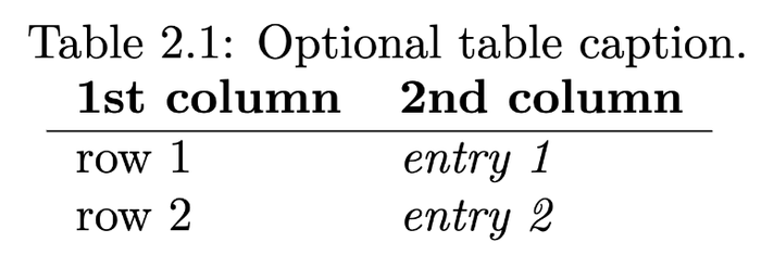
The \begin{tabular} command is always followed by a mandatory set of parameters (here: {ll}). These parameters define the number of columns and the text alignment of each of them (here we defined a two-column table with left-aligned text). You can choose between the following alignment parameters:
| Parameter | Description |
|---|---|
l |
text alignment to the left |
r |
text alignment to the right |
c |
centered text |
Horizontal separators can be achieved by placing a horizontal line command \hline at the end of the desired table row. Alternatively, you can use \toprule, \bottomrule and \midrule for enhanced line layouts.
Vertical separators between the columns can be achieved by placing a perpendicular line | between the parameters listed above (e.g., \begin{tabular}{l|l}). Vertical separators within a cell can be achieved by placing a vertical line command \vline at the desired position within the cell.
\\ indicates a linebreak and hence a new row within the table environment.
Placement of the table: For tables, the same optional placement parameters (\begin{table}[option]) apply as for images.
Labeling: For tables, the same rules for the labeling command (\label{label_name}) apply as for images.
Online table generators like tablesgenerator.com ꜛ are useful tools that help to create (especially huge) tables.
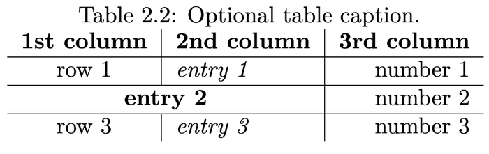
Combining columns
The \multicolumn{number}{alignment}{cell content} command combines several columns within one row while keeping the remaining rows untouched:
{number} |
the number of columns to be combined |
{alignment} |
text alignment of the resulting combined cell |
{cell content} |
the cell entry of the resulting combined cell |
\begin{table}[!b]
  \centering
    \caption{Optional table caption.}
    \begin{tabular}{c|l|r}
      \textbf{1st column} & \textbf{2nd column} & \textbf{3rd column}\\ \hline
      row 1 & \textit{entry 1} & number 1\\ \hline
      \multicolumn{2}{c|}{\textbf{entry 2}} & number 2\\ \hline
      row 3 & \textit{entry 3} & number 3\\
    \end{tabular}
    \label{tab:my_label}
\end{table}
Reserved characters and backslash masking
The following characters are reserved for $\LaTeX$-commands:
| Character | Description |
|---|---|
\ |
initializes a command |
{ } |
embraces arguments of a command |
[ ] |
embraces optional command parameters |
% |
initializes a comment |
& |
separates columns in tables or serves as an alignment marker in eqnarray or align |
# |
parameter for own command declarations |
_ |
initializes a subscript in math mode |
^ |
initializes a superscript in math mode |
In order to use any of these characters withing your text, you need to mask it with a backslash \, e.g. $\[0, 1\]$ for [0, 1]. If you want to display a backslash, \\ won’t work as this is reserved for linebreaks. Instead, use \textbackslash. In math mode, you don’t need to put the extra backslash.
Maths
The following lists contain some common and hence frequently used mathematical symbols, functions and expressions. For a broader and more complete overview, please check the further reading list below. All symbols and functions only work in math mode.
Missing predefined function: With the \operatorname{name}(argument) command you can define your own function, e.g. $\operatorname{tr}(A)$.
Markdown: All math mode commands covered by the default $\LaTeX$ and the amsmath packages can also be used in Markdown documents. In this post, you can read how to enable $\LaTeX$ via MathJax in your Markdown processor.
Equations
In \(\LaTeX\), mathematical expressions can be presented in two ways: as an inline expression in the middle of a sentence or as a display style equation in its own paragraph:
- Inline expressions can be generated by placing a dollar sign
$around the expression, e.g.,$E=\frac{1}{2}nk_BT$generates \(E=\frac{1}{2}nk_BT\), or by placing the epxression between the signs\(and\), e.g.,\(E=\frac{1}{2}nk_BT\). - Display style equations can be generated by placing two dollar sign
$$around the expression or by placing the expression between the signs\[and\], e.g.,\[E=\frac{1}{2}nk_BT\]generates \[E=\frac{1}{2}nk_BT\]
For automatically enumerated equation, use the extended equation command:
\begin{equation}
  E=\frac{1}{2}nk_BT
\end{equation}
If you prefer the extended equation command, but you want to suppress the equation number, just add an asterisks * to equation (this solution also applies to all following commands):
\begin{equation*}
  E=\frac{1}{2}nk_BT
\end{equation*}
For multi-line equations, either use the eqnarray or the align command:
\begin{eqnarray}
  E_{kin} &=& E_{pot} \\
  \Leftrightarrow   \frac{1}{2} m v^2 &=& \frac{GMm}{r}  \\
  \Leftrightarrow   v  &=& \sqrt{ 2 \frac{GM}{r}} := v_{escape}
\end{eqnarray}
\begin{align}
  E_{kin} &= E_{pot} \\
  \Leftrightarrow \frac{1}{2} m v^2 &= \frac{GMm}{r}  \\
  \Leftrightarrow v  &= \sqrt{ 2 \frac{GM}{r}} := v_{escape}
\end{align}
Note that the & sign serves as an alignment marker for vertical alignment within your set of equations. One difference (among others ꜛ) between eqnarray and align is that for align, only one alignment marker is required instead of two for eqnarray.
The amsmath and amssymb packages: The align command as well as many other mathematical commands shown in this guide are part of the amsmath and amssymb package and you need to include them via \usepackage{amsmath} and \usepackage{amssymb} in the preamble of your $\LaTeX$ document.
math mode: Both, the inline and the display style environment are $\LaTeX$’s so-called math mode, which separates mathematical expressions from the main text. Mathematical markups and Greek and special characters only work in this math mode.
\\ performs a linebreak and hence a new row within the eqnarray and align environment. Read more about linebreaks in this section.
\notag suppresses the numbering of a single line within the eqnarray and align environment.
Mathematical symbols
| Symbol | Command | Description | |
|---|---|---|---|
| $+$ | + |
addition | |
| $-$ | - |
subtraction | |
| $\pm$, $\mp$ | \pm, \mp |
plus or minus | |
| $\times$ | \times |
multiplication (times) | |
| $\cdot$ | \cdot |
multiplication (dot) | |
| $\div$, $/$ | \div, / |
division | |
| $\oplus$, $\otimes$ | \oplus, \otimes |
circle plus and circle times | |
| $\circ$ | \circ |
circle | |
| $\bullet$ | \bullet |
filled circle | |
| $=$ | = |
equal | |
| $\ne$ | \ne |
not equal | |
| $<$ | < |
less than | |
| $>$ | > |
greater than | |
| $\ll$ | \ll |
much less than | |
| $\gg$ | \gg |
much greater than | |
| $\le$ | \le |
less than or equal to | |
| $\le$ | \ge |
greater than or equal to | |
| $\approx$ | \approx |
approximately equal to | |
| $\sim$, $\propto$ | \sim, \propto |
similar/proportional to | |
| $\infty$ | \infty |
infinity | |
| $\ldots$ | \ldots |
lower horizontal dots | |
| $\cdots$ | \cdots |
centered horizontal dots | |
| $\vdots$ | \vdots |
vertical dots | |
| $|x|$ | |x| |
absolute value | |
| $\perp$ | \perp |
perpendicular | |
| $\parallel$ | \parallel |
parallel | |
| $\hat a$ | \hat a |
hat | |
| $\widehat{AAA}$ | \widehat{AAA} |
wide hat | |
| $\overset{!}{=}$ | \overset{!}{=} |
overset | |
| $\equiv$ | \equiv |
equivalence relation | |
| $\underset{n=0}{\rightarrow}$ | \underset{n=0}{\rightarrow} |
underset | |
| $x\underset{n\rightarrow0}{\underbrace{=}}\infty$ | x\underset{n\rightarrow0}{\underbrace{=}}\infty |
underset and underbrace | |
| $\square$ | \square |
square | |
| $\blacksquare$ | \blacksquare |
filled square, quod erat demonstrandum (qed/q.e.d.) | |
| $\stackrel{!}{=}$ | \stackrel{!}{=} |
overlay signs with text |
Set of numbers:
| Symbol | Command | Description |
|---|---|---|
| $\mathbb{N}$ | \mathbb{N} |
natural numbers |
| $\mathbb{Z}$ | \mathbb{Z} |
integers numbers |
| $\mathbb{Q}$ | \mathbb{Q} |
rational numbers |
| $\mathbb{R}$ | \mathbb{R} |
real numbers |
| $\mathbb{C}$ | \mathbb{C} |
complex numbers |
Arrows:
| Symbol | Command |
|---|---|
| $\rightarrow$, $\leftarrow$ | \rightarrow, \leftarrow |
| $\Rightarrow$, $\Leftarrow$ | \Rightarrow, \Leftarrow |
| $\Leftrightarrow$, $\leftrightarrow$ | \Leftrightarrow, \leftrightarrow |
| $\longrightarrow$, $\longleftarrow$ | \longrightarrow, \longleftarrow |
| $\Longrightarrow$, $\Longleftarrow$ | \Longrightarrow, \Longleftarrow |
| $\uparrow$, $\downarrow$ | \uparrow, \downarrow |
| $\Uparrow$, $\Downarrow$ | \Uparrow, \Downarrow |
| $\rightrightarrows$, $\leftleftarrows$ | \rightrightarrows, \leftleftarrows |
| $\rightleftarrows$, $\leftrightarrows$ | \rightleftarrows, \leftrightarrows |
| $\rightleftharpoons$, $\leftrightharpoons$ | \rightleftharpoons, \leftrightharpoons |
Calculus
| Function | Command | Description |
|---|---|---|
| $\sqrt{x}$ | \sqrt{x} |
square root |
| $\sqrt[n]{x}$ | \sqrt[n]{x} |
$n$th root |
| $a^b $ | a^b |
superscript |
| $a_b$ | a_b |
subscript |
| $\displaystyle\sum_{n=1}^{\infty}a_n$ | \sum_{n=1}^{\infty}a_n |
summation |
| $\displaystyle\prod_{n=1}^{\infty}a_n$ | \prod_{n=1}^{\infty}a_n |
product |
| $\displaystyle\lim_{x\to \infty}$ | \lim_{x\to \infty} |
limits |
| $\frac{a}{b}$ | \frac{a}{b} |
fraction |
| $\mathrm{d} x$ | \mathrm{d} x |
differential |
| $\partial$ | \partial |
partial |
| $\dot a$, $\ddot a$ , $\dddot a$ | \dot a, \ddot a, \dddot a |
first, second and third temporal derivative |
| $\displaystyle\int\limits_a^b x^2\; \mathrm{d}x$ | \int\limits_a^b x^2\; \mathrm{d}x |
integral |
| $\iint$ | \iint |
double integral |
| $\iiint$ | \iiint |
tripple integral |
| $\oint$ | \oint |
circulation |
| $\nabla$ | \nabla |
Nabla operator |
| $\Delta$ | \Delta |
Laplace operator |
| $\exp(x)$ | \exp(x) |
exponential of $f$ |
| $\ln(x)$ | \ln(x) |
natural logrithm |
| $\log_{a}b$ | \log_{a}b |
logarithm of $b$ to the base $a$ |
Linear algebra
| Function | Command | Description |
|---|---|---|
| $\vec{v}$, $\mathbf{v}$ | \vec{v}, \mathbf{v} |
vector |
| $||\vec{v}||$ | ||\vec{v}|| |
norm |
| $\mathbf{A}$, $\underline{\underline{A}}$ | \mathbf{A}, \underline{\underline{A}} |
matrix |
| $\det$ | \det |
determinant |
| $\dim(V)$ | \dim(V) |
dimension |
| $\operatorname{tr}(A)$ | \operatorname{tr}(A) |
trace of $A$ |
Determinant:
\left|
  \begin{array}{ccc}
      3 & 2 & 1 \\
      6 & 5 & 4 \\
      0 & 8 & 7
  \end{array}
\right|
Piecewise function:
|x| = \begin{cases}
        x,  & \text{for}\; x \ge 0 \\
        -x  & \text{for}\; x = 0
      \end{cases}
Matrices:
\left[
  \begin{array}{ccc}
      3 & 2 & 1 \\
      6 & 5 & 4 \\
      0 & 8 & 7
  \end{array}
\right]
Predefined matrices of the amsmath package: Include the amsmath package in your preamble (\usepackage{amsmath}) in order to use one of the following predefined matrices:
| Matrix type | Surrounding delimeter |
|---|---|
pmatrix |
$(\;)$ |
bmatrix |
$[\;]$ |
Bmatrix |
{$\;$} |
vmatrix |
$|\;|$ |
Vmatrix |
$||\;||$ |
For example:
$
A_{m,n} =
\begin{bmatrix}
  a_{1,1} & a_{1,2} & \cdots & a_{1,n} \\
  a_{2,1} & a_{2,2} & \cdots & a_{2,n} \\
  \vdots  & \vdots  & \ddots & \vdots  \\
  a_{m,1} & a_{m,2} & \cdots & a_{m,n}
\end{bmatrix}
$
Read more about matrices in $\LaTeX$, e.g., hereꜛ.
Geometry and trigonometry
| Function | Command | Description |
|---|---|---|
| $\sin$ | \sin |
sine |
| $\cos$ | \cos |
cosine |
| $\tan$ | \tan |
tangent |
| $\cot$ | \cot |
cotangent |
| $\sec$ | \sec |
secant |
| $\sinh$ | \sinh |
hyperbolic sine |
| $\cosh$ | \cosh |
hyperbolic cosine |
| $\tanh$ | \tanh |
hyperbolic tangent |
| $\csc$ | \csc |
hyperbolic cosecant |
| $\arcsin$ | \arcsin |
area sine |
| $\arccos$ | \arccos |
area cosine |
| $\arctan$ | \arctan |
area tangent |
| $\angle ABC$ | \angle ABC |
angle |
| $\deg(f)$ | \deg(f) |
degree of $f$ |
| $\triangle ABC$ | \triangle ABC |
triangle |
| $\overline{ABC}$ | \overline{ABC} |
segment |
| $5^\circ$ | 5^\circ |
$5$ degree |
Set theory
| Function | Command | Description |
|---|---|---|
| $\min$ | \min |
minimum |
| $\max$ | \max |
maximum |
| $\sup$ | \sup |
supremum |
| $\inf$ | \inf |
infimum |
| $\limsup$ | \limsup |
limit superior |
| $\liminf$ | \liminf |
limit inferior |
| $\overline{A}$ | \overline{A} |
closure |
| $\lbrace{1,2,3\rbrace}$ | \lbrace{1,2,3\rbrace} or \{1,2,3\} |
set brackets |
| $\in$ | \in |
element of |
| $\not\in$ | \not\in |
not an element of |
| $\subset$, $\subseteq$ | \subset, \subseteq |
subset of |
| $\not\subset$ | \not\subset |
not a subset of |
| $\supset$, $\supseteq$ | \supset, \supseteq |
contains |
| $\cup$ | \cup |
union |
| $\cap$ | \cap |
intersection |
| $\bigcup_{n=1}^{10}A_n$ | \bigcup_{n=1}^{10}A_n |
big union |
| $\bigcap_{n=1}^{10}A_n$ | \bigcap_{n=1}^{10}A_n |
big intersection |
| $\emptyset$, $\varnothing$ | \emptyset, \varnothing |
empty set |
| $\mathcal{P}$ | \mathcal{P} |
power set |
Boolean operators
| Function | Command | Description |
|---|---|---|
| $\neg$ | \neg |
not |
| $\land$ | \land |
and |
| $\lor$ | \lor |
or |
| $\implies$ | \implies |
if…then |
| $\equiv$ | \equiv |
if and only if |
| $\therefore$ | \therefore |
therefore |
| $\exists$ | \exists |
there exists |
| $\nexists$ | \nexists |
there not exists |
| $\forall$ | \forall |
for all |
Delimeters
To make delimiters ((), [], {}) large enough to fit the enclosed mathematical expression, add the commands \left and \right next to the delimiters, e.g.:
\left[ \frac{(1-x)}{n} \right]^{0.5}
Physical units
In order to display physical units within text corectly, you can use the siunitx package (\usepackage{siunitx}), which provides the following commands:
| Command | Description |
|---|---|
\num{number} |
correct representation of a given number |
\si{unit} |
helper function to display SI units |
\SI{number}{unit} |
combination of the previous two commands |
For example:
| Command | Output | |
|---|---|---|
| siunitx: manual: |
\num{6.9845e67}$6.9845\,\times\,10^{67}$ |
$6.9845\;\times\;10^{67}$ |
| siunitx: manual: |
[g] = \si{\meter \per \second \squared}$[g] = \textrm{m}\,\textrm{s}^{-2}$ |
$[g] = \textrm{m}\,\textrm{s}^{-2}$ |
| siunitx: manual: |
E = \SI{1.3}{\kilo\volt\per\milli\meter}$E = 1.3 \frac{\textrm{kV}}{\textrm{mm}}$ |
$E = 1.3 \frac{\textrm{kV}}{\textrm{mm}}$ |
Greek alphabet
| Letter | Command | Letter | Command |
|---|---|---|---|
| $\alpha$ | \alpha |
$\nu$ | \nu |
| $\beta$ | \beta |
$\Xi$, $\varXi$, $\xi$ | \Xi, \varXi, \xi |
| $\Gamma$, $\varGamma$, $\digamma$, $\gamma$ | \Gamma, \varGamma,\digamma, \gamma |
$\Pi$, $\varPi$, $\pi$, $\varpi$ | \Pi, \varPi,\pi, \varpi |
| $\Delta$, $\delta$ | \Delta, \delta |
$\rho$, $\varrho$ | \rho, \varrho |
| $\epsilon$, $\varepsilon$ | \epsilon, \varepsilon |
$\Sigma$, $\varSigma$, $\sigma$, $\varsigma$ | \Sigma, \varSigma,\sigma, \varsigma |
| $\zeta$ | \zeta |
$\tau$ | \tau |
| $\eta$ | \eta |
$\Upsilon$, $\varUpsilon$, $\upsilon$ | \Upsilon, \varUpsilon,\upsilon |
| $\Theta$, $\varTheta$, $\theta$, , $\vartheta$ | \Theta, \varTheta,\theta, \vartheta |
$\Phi$, $\varPhi$, $\phi$, $\varphi$ | \Phi, \varPhi,\phi, \varphi |
| $\iota$ | \iota |
$\chi$ | \chi |
| $\kappa$, $\varkappa$ | \kappa, \varkappa |
$\Psi$, $\varPsi$, $\psi$ | \Psi, \varPsi, \psi |
| $\Lambda$, $\varLambda$, $\lambda$ | \Lambda, \varLambda,\lambda |
$\Omega$, $\varOmega$, $\omega$ | \Omega, \varOmega,\omega |
| $\mu$ | \mu |
Special letters
| Letter | Command | Meaning |
|---|---|---|
| $\hbar$ | \hbar |
$\frac{h}{2\pi}$ with $h$ as Planck’s constant ꜛ |
| $\eth$ | \eth |
eth symbol |
| $\surd$ | \surd |
radical or root sign |
| $\Re$ | \Re |
real part |
| $\Im$ | \Im |
imaginary part |
| $\mathrm{e}$ | \mathrm{e} |
Euler’s number ꜛ |
| $\mathrm{i}$ | \mathrm{i} |
imaginary unit ꜛ |
| $\mathcal{O}$ | \mathcal{O} |
Landau symbol ꜛ (big O notation) |
| © | \copyright |
Copyright sign |
| ® | \textregistered |
Registered sign |
Usage in Markdown: All Greek and special characters can be used in Markdown, except the Copyright and Registered sign (insert them in Markdown via © and ®, respectively).
Directories
Bibliography
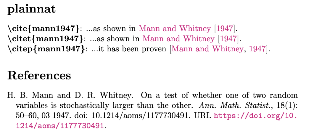
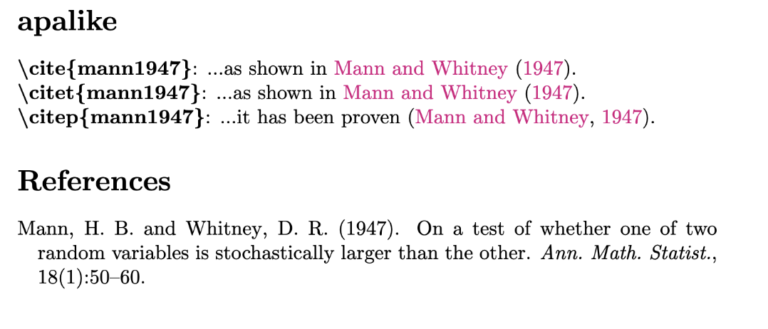
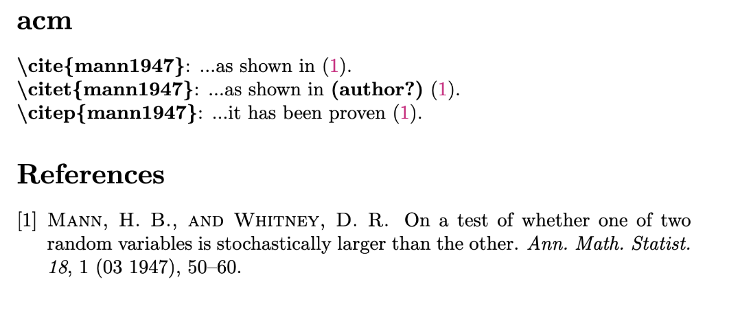
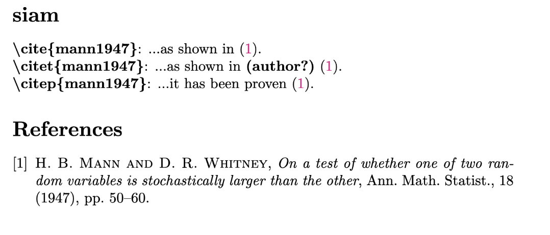
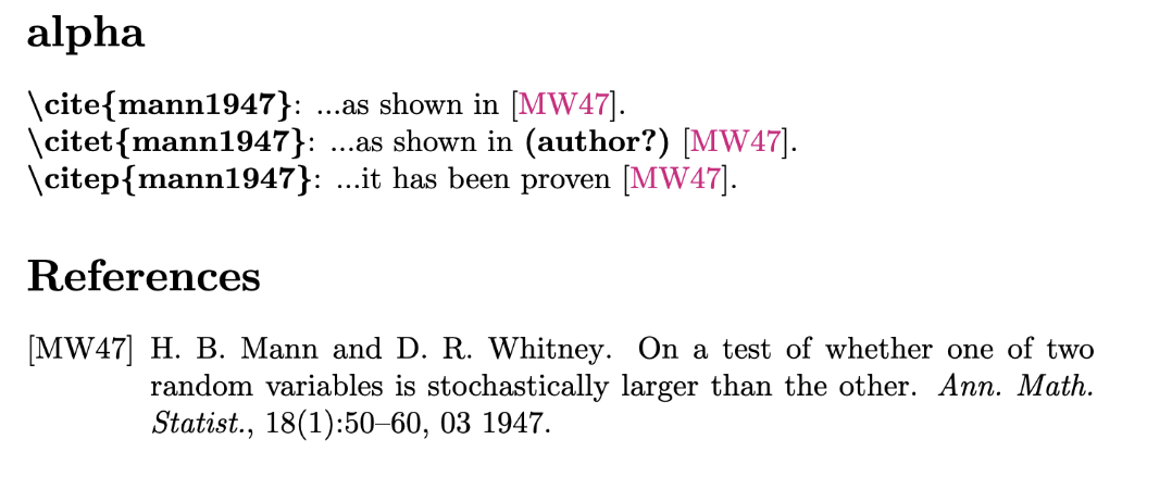
Include the natbib package in your preamble (\usepackage{natbib}). At the end of your document (but before \end{document}), place the command \bibliographystyle{choose_a_style} and fill in the placeholder choose_a_style one of the following bibliography styles:
| bibliography style | Example |
|---|---|
plainnat, abbrvnat |
 |
apalike |
 |
plain, abbrv |
 |
acm |
 |
siam |
 |
alpha |
 |
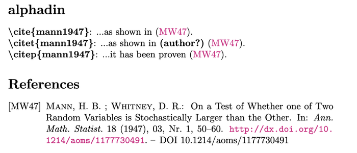
alphadin |
 |
After the \bibliographystyle command, place the command \bibliography{path_to_your_BibTeX_file} and replace the placeholder path_to_your_BibTeX_file with the file path to your BibTeX file ꜛ.
Now you can cite the references listed in your BibTeX file. Use one of the following commands to insert a citation and use the exact cite key of each reference within your BibTeX file:
| Citation command | Output example |
|---|---|
\cite{Gurnett2007} |
Gurnett et al. (2007) |
\citet{Gurnett2007} |
Gurnett et al. (2007) |
\citep{Gurnett2007} |
(Gurnett et al., 2007) |
\citet[see p. 3]{Gurnett2007} |
Gurnett et al. (2007, see p. 3) |
\citep[see p. 3]{Gurnett2007} |
(Gurnett et al., 2007, see p. 3) |
\citeauthor{Gurnett2007} |
Gurnett et al. |
\citeyear{Gurnett2007} |
2007 |
\citeyearpar{Gurnett2007} |
(2007) |
\citealt{Gurnett2007} |
Gurnett et al. 2007 |
\citealp{Gurnett2007} |
Gurnett et al., 2007 |
\citetext{priv.\ comm.} |
(priv. comm.) |
\nocite{Gurnett2007} |
Reference will only appear in your bibliography but not in your main text |
An example file including all commands would look like:
\documentclass{article}
\usepackage{natbib}
\begin{document}

\citet{Gurnett2007} showed, that...

\bibliographystyle{plainnat}
\bibliography{path_to_your_BibTeX_file}
\end{document}
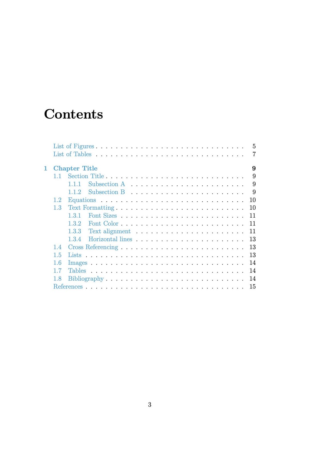
Table of contents
Add the command \tableofcontents right after the \begin{document} command to generate a table of contents. In the preamble, you can specify the displayed depth of the table of contents via the \setcounter command:
\documentclass[14pt]{article}
\setcounter{tocdepth}{3}

\begin{document}
\tableofcontents

\section{Some title}
My contents...

\end{document}
Manually adding entries to the table of contents can be achieved via the \addcontentsline{toc}{toc_level}{entry_name}, e.g., place the command \addcontentsline{toc}{section}{References} right after the \bibliography{path_to_your_BibTeX_file} command to add your bibliography to your table of contents on section level with the name “References”.
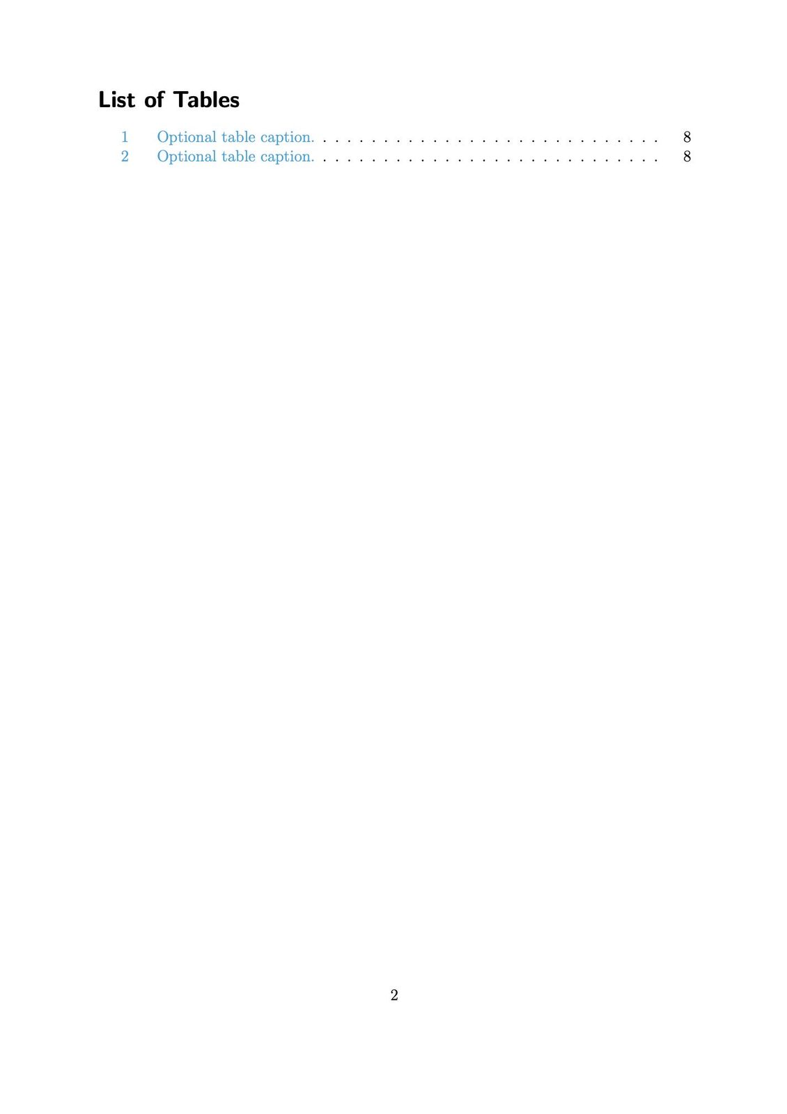
List of figures and tables
Similar to the table of contents insertion, place the commands \listoffigures and \listoftables at the beginning or th end of your document to generate a list of figures and list of tables, respectively, used in your document:
\documentclass[14pt]{book}

\begin{document}

% add a table of contents:
\tableofcontents

% add a list of figures:
\listoffigures
\addcontentsline{toc}{chapter}{List of Figures}

% add a list of tables:
\listoftables
\addcontentsline{toc}{chapter}{List of Tables}

% start of my main content:
\chapter{Some title}
My contents...

\end{document}
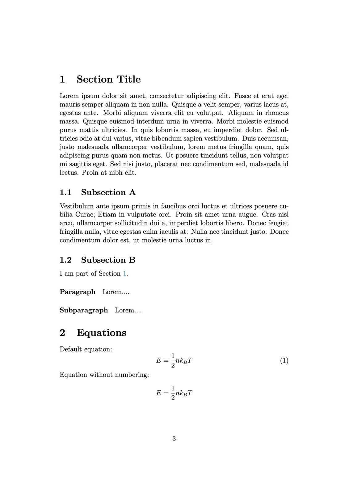
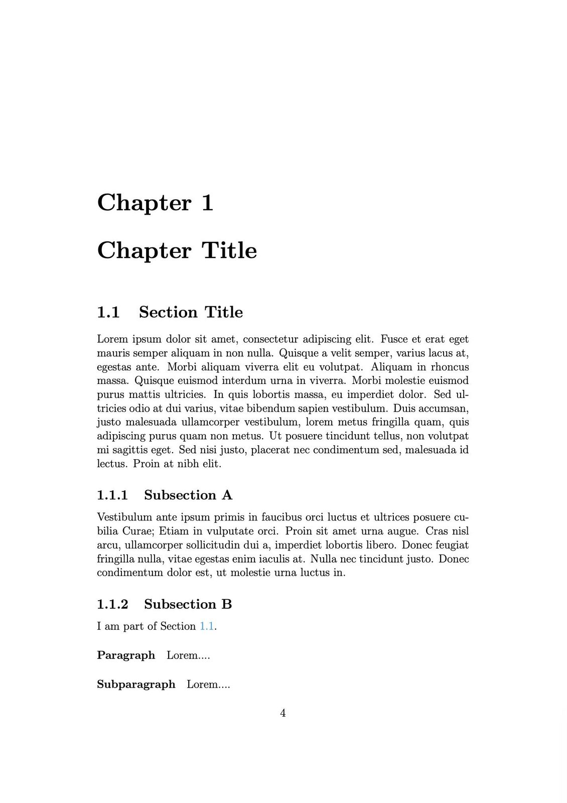
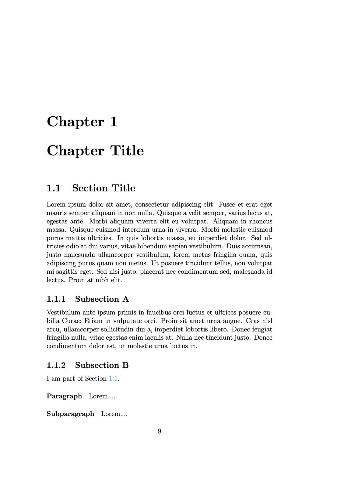
Examples
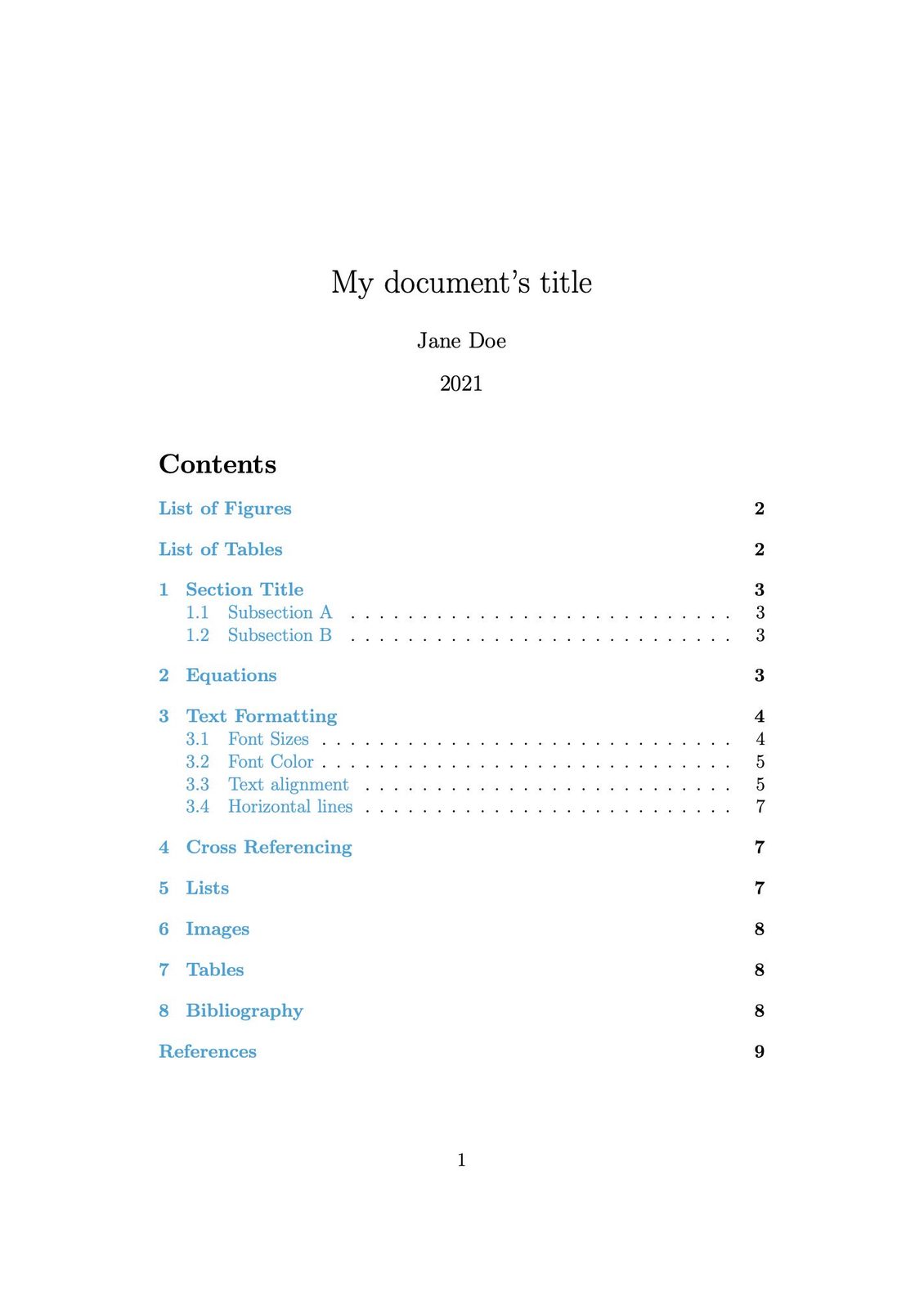
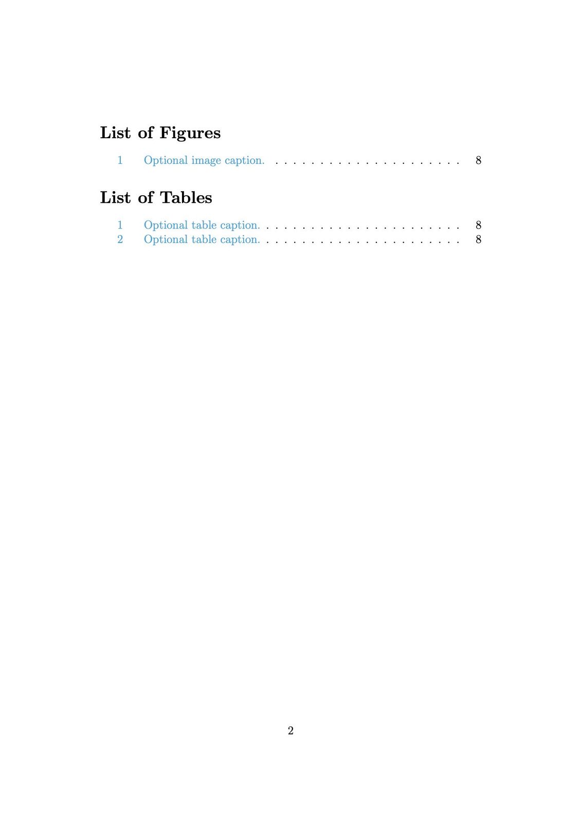
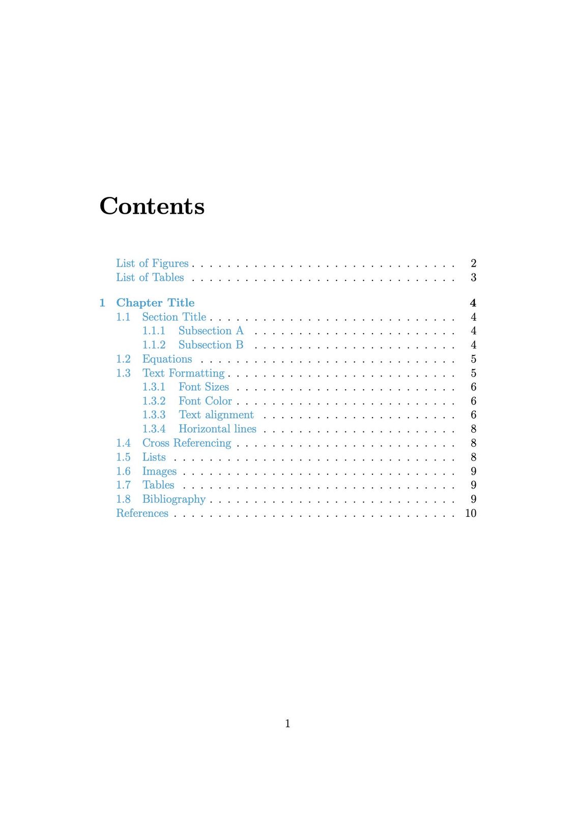
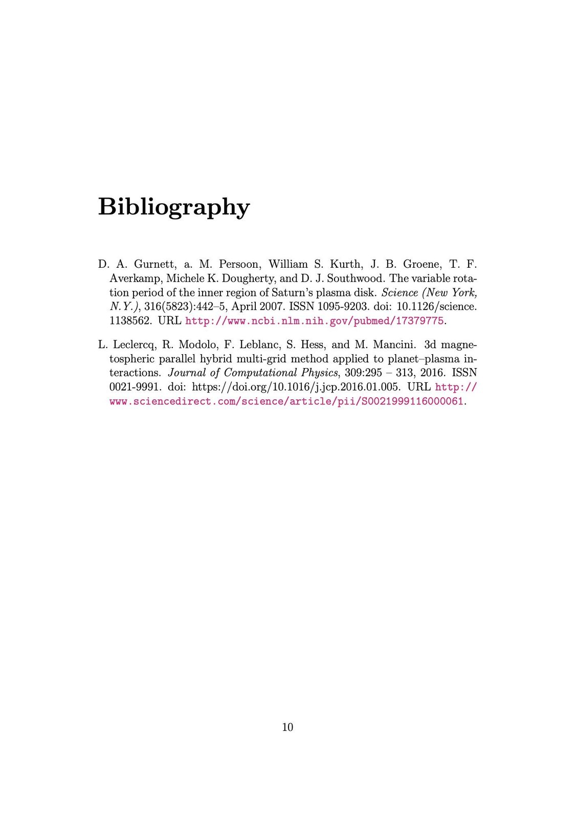
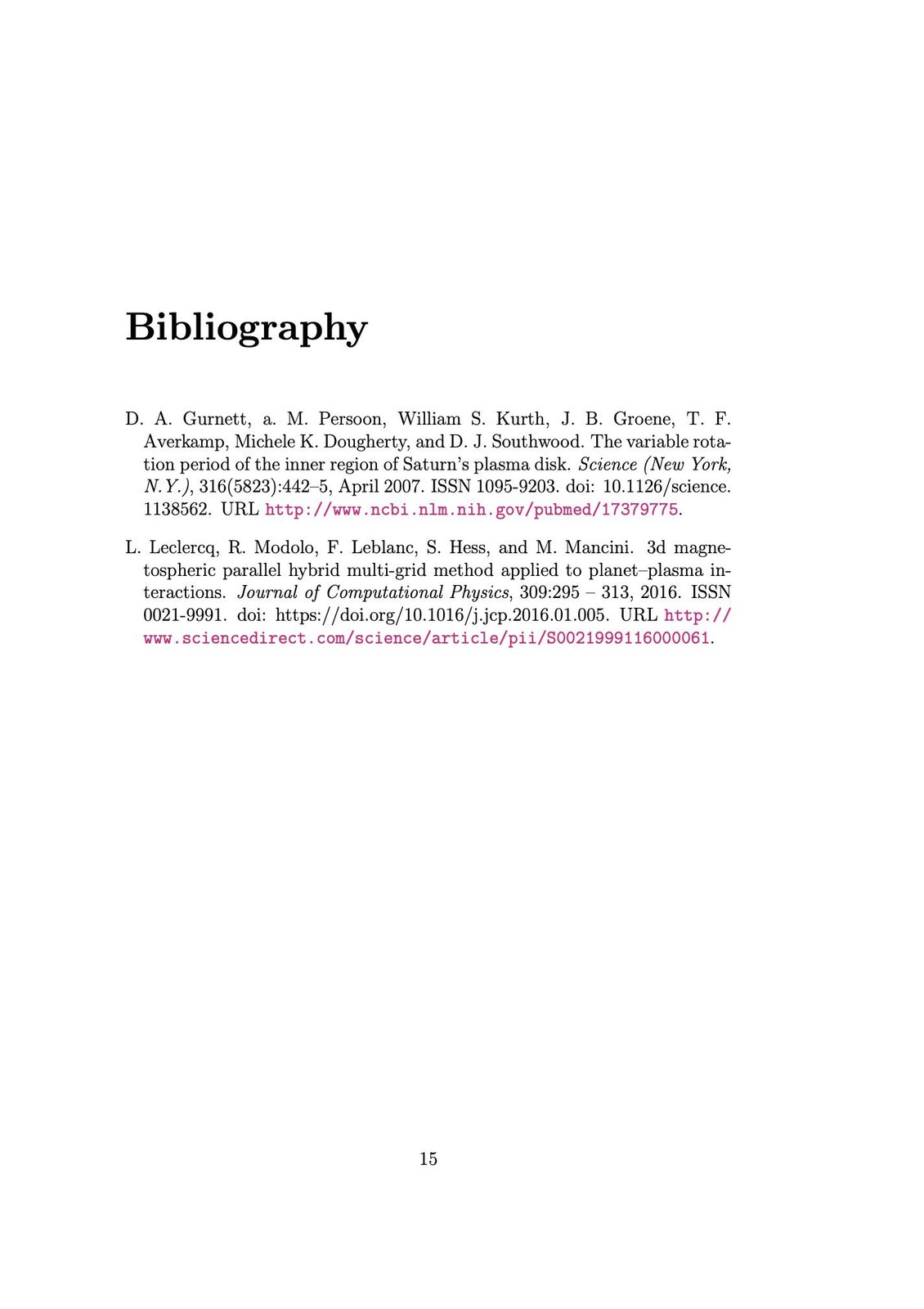
In the following, you see the final outputs of a LaTeX document, that contains almost all examples shown above. The document has been compiled for different document classes to demonstrate the differences among them.
Comparing the article class (left), report class (middle), and book class (right):


Comparing the equivalent Koma script classes scrartcl class (left), scrrprt class (middle), and scrbook class (right):
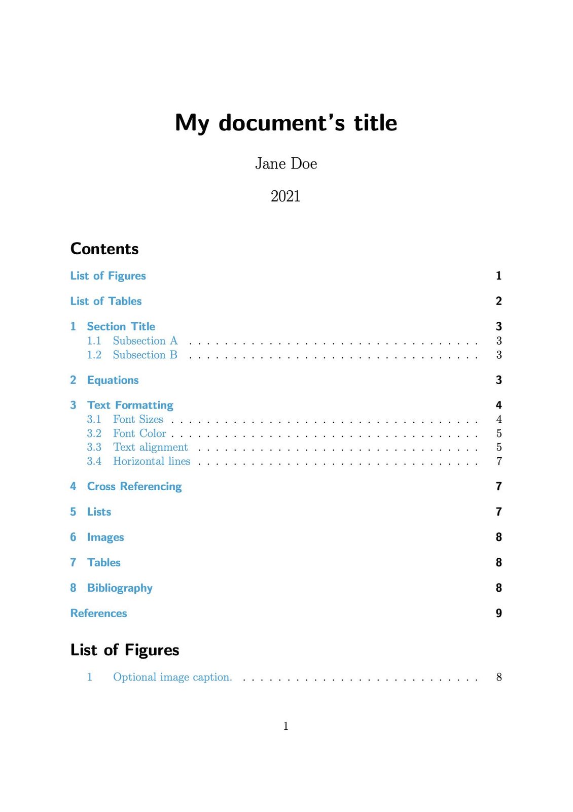


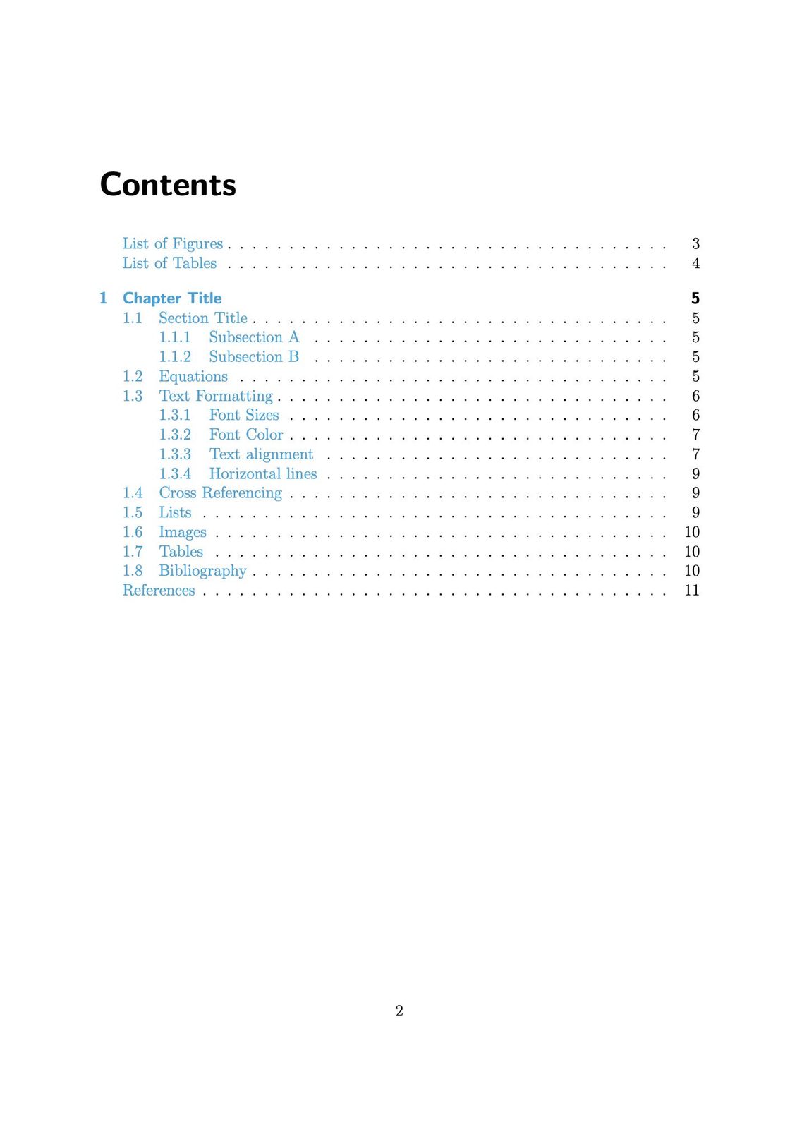
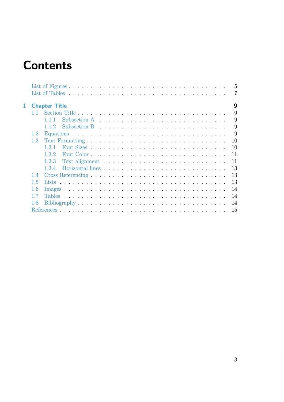
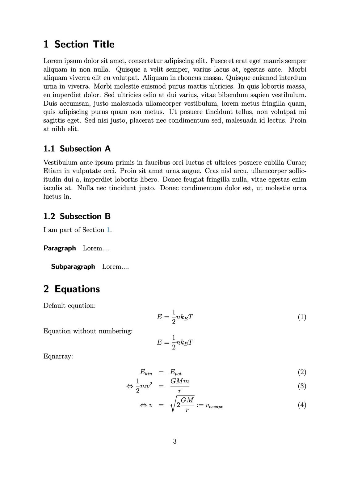
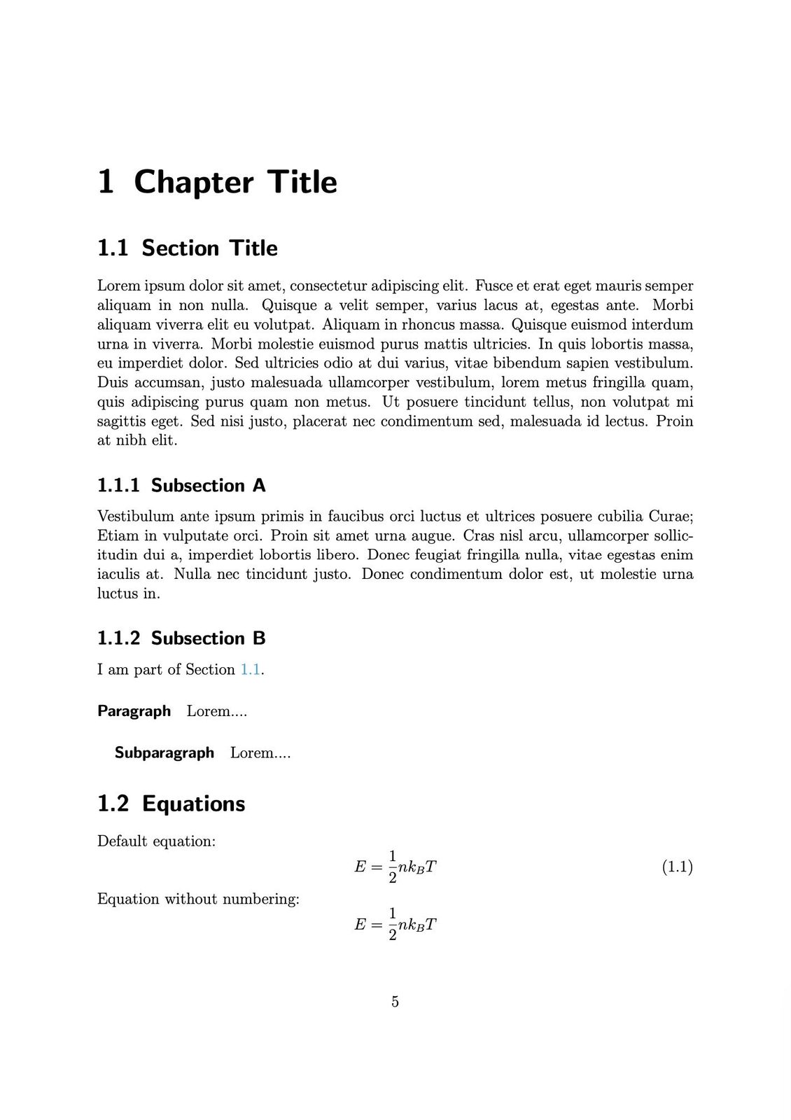
The most prominent differences are between the article/scrartcl and report/scrrprt classes. The report/scrrprt and book/scrbook classes share an almost similar layout, except that the book/scrbook classes are designed for a two-sided page layout by default (i.e., alternating margins on the left and right side). The major difference between the default and the Koma script classes is a more modern looking layout in the latter ones. Not shown and discussed here are also several more and quite useful options that come with Koma script classes.
You can download the Latex file and the used example BibTeX file as well as the output PDF here:
- LatTeX testings.tex
- BibTeX.bib
- pixel_tracker_logo_120px.jpg
- LatTeX testings (article).pdf
- LatTeX testings (scrartcl).pdf
- LatTeX testings (report).pdf
- LatTeX testings (scrreprt).pdf
- LatTeX testings (book).pdf
- LatTeX testings (scrbook).pdf
References and further readings
The main source thankfully used to generate this guide are:
Further readings
- Tutorial website on general $\LaTeX$ usage: overleaf.com/learn ꜛ
- CTAN: The Comprehensive TEX Archive Network ꜛ
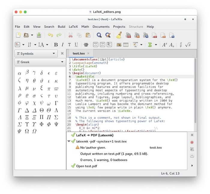
- A list of freely available $\LaTeX$ editors
- Wikipedia article ꜛ on mathematical $\LaTeX$ commands
- Wikipedia article ꜛ on mathematical symbols
- Scott Pakin’s “The Comprehensive $\LaTeX$ Symbol List” ꜛ
- Emanuel Regnath’s ꜛ “LaTeX Mathematical Symbols” ꜛ
- Wikipedia article ꜛ on $\LaTeX$’s bibliography management
- Usage of $\LaTeX$ commands in Markdown documents
- How to enable $\LaTeX$ in Markdown documents
- Markdown vs. $\LaTeX$ for Scientific Writing

This work is licensed under a Creative Commons Attribution-NonCommercial-ShareAlike 4.0 International License (CC BY-NC-SA 4.0) ꜛ.


