Spike inference from Calcium imaging data with CASCADE

CASCADE, short for Calibrated spike inference from calcium imaging data using deep networks, is an open-source, deep learning-based pipeline for inferring neuronal spike trains from calcium imaging data. It provides robust and calibrated spike inference by leveraging ground truth datasets and convolutional neural networks, enabling the reconstruction of neuronal spiking activity from noisy or slow calcium fluorescence signals.

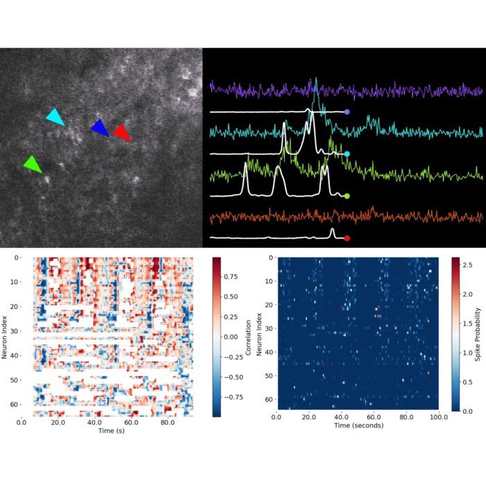
CASCADE translates calcium imaging $\Delta F/F$ traces into spiking probabilities or discrete spikes. Source: CASCADE GitHub repositoryꜛ (license: MIT License)

CASCADE operates by first training on large-scale ground truth data, then applying a pre-trained or custom model to new experimental calcium traces, thereby generating probabilistic or discrete spike estimates.

The approach is particularly valuable for neuroscience experiments where direct electrophysiological recordings are impractical, and offers a standardized, reproducible method for analyzing large calcium imaging datasets.

Acknowledgment

This script is entirely based on the official demoꜛ provided by the CASCADE teamꜛ, with modifications for use in the present course. Original code by Peter Rupprechtꜛ and Adrian Hoffmannꜛ, Helmchen Labꜛ, in collaboration with the Friedrich Labꜛ. All credit for the original development and maintenance of CASCADE belongs to the authors. For scientific use, please cite the following publication:

Rupprecht et al., A database and deep learning toolbox for noise-optimized, generalized spike inference from calcium imaging, 2021, Nature Neuroscience, DOI: 10.1038/s41593-021-00895-5ꜛ.

Please refer to the CASCADE GitHub repositoryꜛ for the latest updates, documentation, and contact information. Feedback regarding this adaptation may be directed to the course instructor; questions about CASCADE itself should be addressed to Peter Rupprechtꜛ.

Installation

Before you begin, ensure that that you have installed the latest version of Miniforgeꜛ on your computer. Miniforge is a minimal installer for conda, which is a package manager that allows you to install Python packages and their dependencies easily. The latest versions come with the mamba package manager, which is a faster alternative to conda. If you are using an older version of Miniforge, you can use conda instead of mamba and install mamba in your new environment separately. Follow similar steps as described in the previous tutorial.

Create a conda environment with CASCADE

First, we need to create a conda environment with the required packages. CASCADE offers instructions for different platforms, including Windows, macOS, and Linux, with and without GPU support:

PC (Windows/Linux) with GPU support

For a GPU installation (faster, recommended if you will train networks):

mamba create -n cascade python=3.7 tensorflow-gpu keras h5py numpy scipy matplotlib seaborn ruamel.yaml ipykernel ipython -c conda-forge -c anaconda -y
mamba activate cascade

PC (Windows/Linux) without GPU support

For a CPU installation (slower, recommended if you will not train a network):

mamba create -n cascade python=3.7 tensorflow keras h5py numpy scipy matplotlib seaborn ruamel.yaml ipykernel ipython -c conda-forge -c anaconda -y
mamba activate cascade

macOS with GPU support

I’ve recently tested this on a MacBook Pro with an M1 chip, using macOS Sequoya 15.5, and it worked perfectly:

mamba create -n cascade_2025 -y python=3.8 tensorflow keras h5py numpy scipy matplotlib seaborn ruamel.yaml ipykernel ipython -c conda-forge -c anaconda -y
mamba activate cascade_2025
mamba install -c apple tensorflow-deps
pip install tensorflow-macos tensorflow-metal

Troubleshooting: If you receive an error message after executing mamba install -c apple tensorflow-deps, skip this step and proceed with the next one. The installation of tensorflow-macos and tensorflow-metal will still work.

Download the CASCADE repository

CASCADE is not available on PyPI, so you need to download the repository from GitHub. The Github repository contains all custom functions, the ground truth datasets and the pre-trained models. To do so, you have two options:

Option 1: Download the repository as a ZIP file

You can download the repository as a ZIP file from the CASCADE GitHub page. After downloading, extract the ZIP file to the tutorial folder 02 Cascade tutorial in the course directory.

Option 2: Clone the repository using Git

If you have Git installed, you can clone the repository directly into the tutorial folder using the following Python command:

# download Cascade if not present (this may take a while):
import os
if "02 Cascade tutorial" in os.getcwd():
    if not os.path.exists('Cascade'):
        print("Cascade directory not found. Cloning the repository...")
        !git clone https://github.com/HelmchenLabSoftware/Cascade
        print("Cascade repository cloned successfully.")
    else:
        print("Cascade directory already exists.")
    os.chdir('Cascade')
    print(f"Changed directory to {os.getcwd()}")

Relation between action potentials and calcium transients

The action potential is the fundamental electrical event by which neurons communicate. It is a brief, stereotyped change in membrane potential, initiated when synaptic input or external stimulation depolarizes the membrane beyond a threshold.

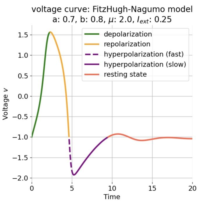
Stages of an action potential. The trace of an action potential can also be simulated numerically, e.g., using the Hodgkin-Huxley or Fitzhugh-Nagumo model. Source: Wikimedia Commons (license: CC BY-SA 3.0; modified)

Phases of the action potential:

• Depolarization: Voltage-gated sodium (Na⁺) channels open, allowing Na⁺ influx and a rapid rise of the membrane potential (from typically −70 mV to +30 mV).
• Repolarization: Sodium channels inactivate; voltage-gated potassium (K⁺) channels open, K⁺ exits the cell, and the membrane potential falls back.
• Hyperpolarization: As K⁺ channels close slowly, the membrane potential briefly undershoots its resting value.

The entire electrical event lasts ~1–2 milliseconds. However, a key link to functional imaging comes from voltage-gated calcium (Ca²⁺) channels, which open during the depolarization (and sometimes early repolarization) phase — most notably at axon terminals and in certain somatic/dendritic compartments. This results in a brief but significant influx of Ca²⁺ ions into the neuron.

Calcium transient:

The influx of Ca²⁺ produces a transient rise in intracellular calcium concentration. The amplitude and time course of this transient depend on:

• The number and timing of action potentials.
• The local density and subtype of Ca²⁺ channels.
• Cellular buffering, extrusion mechanisms, and compartment geometry.

Temporal relationship:

• Action potential: Rapid (1–2 ms, all-or-none, digital signal).
• Ca²⁺ transient: Slower (10–100 ms or more), reflecting biological Ca²⁺ handling.
• Measured fluorescence: Even slower, because the optical signal reflects both the underlying Ca²⁺ dynamics and the kinetics of the chosen indicator (e.g., GCaMP variants, OGB-1, Fluo-4).

Why do indicator kinetics matter?

• Fast indicators (e.g., GCaMP6f) have rapid binding/unbinding and better temporal fidelity, but may have lower signal amplitude.
• Slow indicators (e.g., GCaMP6s) bind Ca²⁺ for longer, producing larger, longer-lasting signals but greater temporal blurring.
• The recorded fluorescence trace is thus a convolution of the cell’s true Ca²⁺ dynamics and the indicator’s own response, resulting in a signal that rises and decays much more slowly than the action potential that triggered it.

Does the fluorescence decay match the true Ca²⁺ decay?

• Not exactly. The decay time of the recorded signal is generally longer than the underlying Ca²⁺ transient because it includes both biological clearance and indicator off-kinetics.
• For this reason, fast and slow indicators exist: to balance sensitivity against temporal resolution, depending on experimental goals.

Summary table:

Event	Typical time course	Notes
Action potential	1–2 ms	Electrical event (Na⁺/K⁺ channels)
Ca²⁺ influx & clearance	10–100 ms (rise/decay)	Biological, varies with cell/compartment
Indicator fluorescence response	50 ms – 1 s (rise/decay)	Convolution of Ca²⁺ + indicator kinetics

Analytical implication:

Calcium imaging does not measure action potentials directly, but a filtered, noisy, and temporally blurred proxy—the fluorescence signal of the indicator bound to Ca²⁺. The lack of strict one-to-one correspondence means:

• Not every spike produces a clearly separable calcium transient (especially at high firing rates or with slow indicators).
• Some calcium transients represent the cumulative effect of multiple spikes.
• Noise, baseline drift, and kinetics can obscure single events.

This biophysical chain underlies the need for careful spike inference algorithms: reconstructing the underlying spike train from the slow, convolved, and noisy optical signal, given known indicator properties and the basic principles of cellular calcium dynamics.

Import required python packages

After this brief background overview, we now begin our analysis and start with importing some standard python packages:

import warnings
import glob
import numpy as np
import scipy.io as sio
import matplotlib.pyplot as plt
import ruamel.yaml as yaml
yaml = yaml.YAML(typ='rt')
warnings.filterwarnings('ignore')

Next, we import modules from the CASCADE folder you just downloaded:

from cascade2p import checks
checks.check_packages()
from cascade2p import cascade # local folder
from cascade2p.utils import plot_dFF_traces, plot_noise_level_distribution, plot_noise_matched_ground_truth

Load a sample data set of $\Delta F/F$ traces

We begin this tutorial with some sample data provided by CASCADE. CASCADE generally expects the traces to be saved as a single large 2D NumPy array, where each row corresponds to a neuron and each column corresponds to a time point (neurons $\times$ time, thus, (neurons, time)). The $\Delta F/F$ values stored therein should be numeric, not in percent (e.g. 0.5 instead of 50%).

To load the sample data, we need to define a function which handles .npy and .mat files (the format used by the sample datasets distributed with CASCADE). This function will read the data and return it as a 2D NumPy array.

Info: If your own data is already in the correct array format, you can skip the usage of this function and use your array directly.

def load_neurons_x_time(file_path):
    """Custom method to load data as 2d array with shape (neurons, nr_timepoints)"""

    if file_path.endswith('.mat'):
      traces = sio.loadmat(file_path)['dF_traces']
      # PLEASE N­OTE: If you use mat73 to load large *.mat-file, be aware of potential numerical errors, see issue #67 (https://github.com/HelmchenLabSoftware/Cascade/issues/67)

    elif file_path.endswith('.npy'):
      traces = np.load(file_path, allow_pickle=True)
      # if saved data was a dictionary packed into a numpy array (MATLAB style): unpack
      if traces.shape == ():
        traces = traces.item()['dF_traces']

    else:
      raise Exception('This function only supports .mat or .npy files.')

    print('Traces standard deviation:', np.nanmean(np.nanstd(traces,axis=1)))
    if np.nanmedian(np.nanstd(traces,axis=1)) > 2:
      print('Fluctuations in dF/F are very large, probably dF/F is given in percent. Traces are divided by 100.')
      return traces/100
    else:
        return traces

Now, we load a sample data set provided by CASCADE. The dataset contains calcium imaging data from a mouse visual cortex, with ground truth spike trains available for comparison. The data is stored in a .mat file, which we will load using the function defined above. We also need to specify the frame rate of the calcium imaging data, which is required for the spike inference process.

example_file = "Example_datasets/Allen-Brain-Observatory-Visual-Coding-30Hz/Experiment_552195520_excerpt.mat"
frame_rate = 30 # fps

# check and load the example file:
try:
  traces = load_neurons_x_time( example_file )
  print('Number of neurons in dataset:', traces.shape[0])
  print('Number of timepoints in dataset:', traces.shape[1])
except Exception as e:
  print('\nSomething went wrong!\nEither the target file is missing, in this case please provide the correct location.\nOr your file is not yet completely uploaded, in this case wait until the upload is completed.\n')
  print('Error message: '+str(e))

# THIS CELL/STEP IS RESERVED FOR THE EXERCISE
# overwrite traces by your own data:
# traces = ...

Let’s investigate the shape of the loaded data to ensure it is in the correct format:

print(f"shape of dF/F traces: {traces.shape}")

The shape (74, 6001) = (neurons $\times$ time) indicates that we have 74 neurons and 6001 time points. So, everything is as expected. Let’s plot the trace of the first neuron to see what it looks like:

# define the neuron index to plot:
neuron_i = 0

# define a time array based on the frame_rate:
time_vector = np.arange(traces.shape[1]) / frame_rate

# plot the calcium trace for the selected neuron:
plt.figure(figsize=(12, 5))
plt.plot(time_vector, traces[neuron_i, :])
plt.xlabel('Time (seconds)')
plt.ylabel(f'\Delta F/F')
plt.xlim(0, time_vector[-1])
plt.title(f'Calcium trace of neuron {neuron_i + 1}')
plt.show()

Trace of the first neuron from the sample dataset. The trace shows the fluorescence signal over time, which is typical for calcium imaging data. The y-axis represents the $\Delta F/F$ values, which indicate changes in fluorescence relative to a baseline level. The x-axis represents time in seconds, based on the specified frame rate of 30 Hz.

Exercise: Plot some other traces to see how they look like. What do you notice?

Instead of plotting a single trace on “our own”, we can use CASCADE’s plotting functions to visualize the traces. This is useful for quickly checking the data quality and understanding the overall structure of the dataset. Here is how you can plot randomly some selected calcium traces:

plt.rcParams['figure.figsize'] = [13, 13]
np.random.seed(0)  # for reproducibility
neuron_indices = np.random.randint(traces.shape[0], size=16)
time_axis = plot_dFF_traces(traces,neuron_indices,frame_rate)

Random sample of calcium traces from the sample dataset. The plot shows the fluorescence signals of 16 randomly selected neurons over time, with each trace representing a different neuron. The y-axis represents the $\Delta F/F$ values, indicating changes in fluorescence relative to a baseline level, while the x-axis represents time in seconds based on the specified frame rate of 30 Hz.

Plotting random traces helps to check whether the data have been loaded correctly. If you want to plot specific instead of randomly selected neurons, modify the variable neuron_indices accordingly.

Plot distribution of noise levels

The traces are quite noisy, which is typical for calcium imaging data.

In calcium imaging analysis, the noise level is a quantitative measure of the baseline variability (fluctuations not caused by neural activity) in each neuron’s fluorescence trace. It is usually given as a standard deviation (or a related metric) of the trace’s background fluctuations, normalized by the signal amplitude and frame rate. CASCADE offers a method to estimate the noise level of the traces:

plt.rcParams['figure.figsize'] = [12, 5]
noise_levels = plot_noise_level_distribution(traces, frame_rate)

Histogram of noise levels across all neurons in the dataset. The x-axis represents the noise level (standard deviation of the fluorescence trace), while the y-axis shows the number of neurons with that noise level. The histogram provides a visual representation of how noise is distributed across the dataset, indicating the variability in signal quality among different neurons.

What does the noise level mean?

• Low noise level: The fluorescence trace has little baseline fluctuation, meaning genuine calcium transients (spikes) stand out more clearly.
• High noise level: The trace is “noisier”, i.e., there are larger random fluctuations not related to neuronal activity, making it harder to reliably detect true events.

Why is this important?

• Quality control: The distribution of noise levels across neurons allows you to assess the overall quality of your dataset. A narrow, low-centered distribution means your data is generally “clean”; a wide or high-centered distribution suggests variable or poor signal quality.
• Spike inference performance: The performance of any spike inference algorithm (including CASCADE) is fundamentally limited by the noise level:
  • Low-noise traces allow more accurate spike detection.
  • High-noise traces may lead to missed spikes (false negatives) or false positives.
• Network training and calibration: CASCADE uses the noise level to select or train an appropriate deep learning model for spike inference, since the ground truth datasets and models are stratified by noise level. For optimal performance, the noise distribution of your data should match that of the ground truth set used to train the model.

What does our noise level histogram tell us?

The histogram above shows how the noise levels are distributed across all neurons in our dataset.

• Peak location: Indicates the typical noise level in our experiment.
• Spread: Reflects neuron-to-neuron variability (possibly due to depth, indicator loading, or other biological/technical factors).
• Outliers: Very high or low noise neurons may warrant further inspection, as they may represent artefacts, poorly segmented cells, or technical errors.

Summary

Computing and visualizing the noise level distribution is a crucial diagnostic step before spike inference. It informs you about data quality, guides model selection, and ultimately sets the fundamental limit on the accuracy of spike train reconstruction from your calcium imaging data.

Prepare CASCADE: Select a pre-trained model

Next, we need to select a pre-trained model for spike inference. CASCADE provides several pre-trained models that are optimized for different noise levels and, of course, different Calcium indicators. Let’s first get a list of available models:

cascade.download_model( 'update_models', verbose = 1)

yaml_file = open('Pretrained_models/available_models.yaml')
X = yaml.load(yaml_file)
list_of_models = list(X.keys())
print('\n List of available models: \n')
for model in list_of_models:
  print(model)

Note: You can view all currently available pre-trained models in the CASCADE GitHub repositoryꜛ.

As you can see, there is already a bunch of pre-trained models available. Instead of scrolling through the list, you can also search for a specific model by its name. For example, if you want to find a model for the GCaMP6 indicator, you can use the following code:

# define some helper function:
import re
def find_models(search_string, model_list):
    
    pattern = re.compile(rf'{search_string}[a-z]*', re.IGNORECASE)
    matching_models = [model for model in model_list if pattern.search(model)]
    if matching_models:
        print(f'\nFound {len(matching_models)} models matching "{search_string}":')
        for model in matching_models:
            print(model)
    else:
        print(f'\nNo models found matching "{search_string}". Please check the spelling or try a different search term.')
    return matching_models

search_string = 'GCaMP6' # search for GCaMP6 models; if you indicator is not listed, try alternative spellings like GC6

# Example usage:
_ = find_models(search_string, list_of_models)

Exercise: Play around with the search function above and search for, e.g., all 15Hz framerate models.

After that, proceed with the next cell. To continue, we select a model that suits best to our sample data set: Global_EXC_30Hz_smoothing25ms. The following code will select and download it:

model_name = "Global_EXC_30Hz_smoothing25ms" 
cascade.download_model(model_name, verbose=1)

Predict spike rates from $\Delta F/F$ traces

The next step is actually the core of the CASCADE pipeline: predicting the spike rates from the $\Delta F/F$ traces using the selected pre-trained model. This step involves passing the calcium fluorescence data through a deep convolutional neural network that has been trained to infer spike rates from similar data.

In the core step of spike inference, CASCADE takes the measured calcium fluorescence traces ($\Delta F/F$) from each neuron and computes an estimate of the underlying spike rate as a function of time. This is achieved by passing sliding windows of the fluorescence data through a deep convolutional neural network that has been trained on ground truth data, where both calcium signals and the true spike times (from simultaneous electrophysiological recordings) are available.

For every time point in the fluorescence trace, CASCADE extracts a temporal window centered on that time point and uses it as input to the neural network. The network then outputs the predicted spike rate for that specific time. In mathematical terms, the model computes

\[\hat{s}(t) = f(\mathbf{F}_{t-w:t+w})\]

where $\hat{s}(t)$ is the estimated spike rate at time $t$, $w$ is the half-width of the temporal window, and $\mathbf{F}_{t-w:t+w}$ is the vector of fluorescence values in a window of length $2w+1$ around time $t$. The function $f$ represents the nonlinear mapping learned by the neural network during training. This operation is repeated for all time points and all neurons in the dataset, producing a continuous-valued time series of estimated spike rates $\hat{s}(t)$ for each neuron.

Computationally, the network performs a complex nonlinear transformation that effectively inverts the convolution and noise corruption introduced by the biophysical calcium indicator. The predicted spike rate reflects the network’s best estimate, given the observed fluorescence and its learned statistical relationship to real spikes, of the probability or intensity of neuronal firing at each time point. This approach is substantially more powerful than simple deconvolution methods because it can account for indicator kinetics, nonlinearities, and noise characteristics learned from training data. The result is a time series for each neuron, in which each value indicates the predicted rate (or probability) of spiking at that moment, thereby transforming the indirect, noisy calcium signal into a direct estimate of neuronal electrical activity suitable for further analysis.

total_array_size = traces.itemsize*traces.size*64/1e9

# If the expected array size is too large for the Colab Notebook, split up for processing
if total_array_size < 1:

  spike_prob = cascade.predict( model_name, traces, verbosity=1 )

# Will only be use for large input arrays (long recordings or many neurons)
else:

  print("Split analysis into chunks in order to fit into Colab memory.")

  # pre-allocate array for results
  spike_prob = np.zeros((traces.shape))
  # nb of neurons and nb of chunks
  nb_neurons = traces.shape[0]
  nb_chunks = int(np.ceil(total_array_size/1))

  chunks = np.array_split(range(nb_neurons), nb_chunks)
  # infer spike rates independently for each chunk
  for part_array in range(nb_chunks):
    spike_prob[chunks[part_array],:] = cascade.predict( model_name, traces[chunks[part_array],:] )

After running the above code, your machine will start processing the calcium traces and predicting the spike rates for each neuron. This may take some time, depending on the size of your dataset and the computational resources available.

Once the processing is complete, you will have a 2D NumPy array spike_prob containing the predicted spike rates for each neuron over time. The shape of this array should match that of the input traces, i.e., (neurons, time):

print(f"Shape of spike probability array: {spike_prob.shape}")

Next, we plot again the calcium trace (traces) of the first neuron, but this time we also plot the inferred spike probability (spike_prob):

neuron_i = 0

# define a time array based on the frame_rate:
time_vector = np.arange(traces.shape[1]) / frame_rate

# plot the calcium trace and the inferred spike probability for the selected neuron:
plt.figure(figsize=(12, 5))
plt.plot(time_vector, traces[neuron_i, :], c="blue", alpha=0.75, label='Calcium trace')
plt.plot(time_vector, spike_prob[neuron_i, :], alpha=0.5, c="orange", label='Inferred spike probability')
plt.xlabel('Time (seconds)')
plt.ylabel(f'\Delta F/F')
plt.xlim(0, time_vector[-1])
plt.ylim(-0.25, 2)
plt.title(f'Calcium trace and inferred spike probability of neuron {neuron_i + 1}')
plt.legend()
plt.show()

Calcium trace and inferred spike probability of the first neuron from the sample dataset. The blue line represents the $\Delta F/F$ values of the calcium trace, while the orange line represents the inferred spike probability over time. The plot allows for visual comparison between the calcium signal and the predicted neuronal activity.

Exercise: Again, play around with the neuron indices variable neuron_i to plot different neurons and assess your results. What do you notice? How well does the inferred spike probability match the calcium trace? Are there any discrepancies or unexpected patterns?

Of course, we can also again use CASCADE’s plotting functions to visualize the traces and the inferred spike probabilities:

N_neurons = 16

neuron_indices = np.random.randint(traces.shape[0], size=N_neurons)
time_axis = plot_dFF_traces(traces,neuron_indices,frame_rate,spike_prob,y_range=(-1.5, 3))

Random sample of calcium traces and inferred spike probabilities from the sample dataset. The plot shows the fluorescence signals of 16 randomly selected neurons over time, with each trace representing a different neuron. The blue lines represent the $\Delta F/F$ values, while the orange lines represent the inferred spike probabilities.

Save predictions to output file

We now have the option, to save our predicted spike probabilities to an output file. Below are a few examples of how to do this:

# create a folder path, that is two levels above the current working directory:
folder_path = os.path.dirname(os.getcwd())
file_name = 'predictions_' + os.path.splitext( os.path.basename(example_file))[0]
save_path = os.path.join(folder_path, file_name)

# save as csv file:
np.savetxt(save_path+'.csv', spike_prob, delimiter=',', fmt='%.6f')

# save as mat file:
#sio.savemat(save_path+'.mat', {'spike_prob':spike_prob})

# save as numpy file:
# np.save(save_path, spike_prob)

Exercise: Load and analyze your own $\Delta F/F$ traces

Now it’s time, the load and plot $\Delta F/F$ traces we have derived from our CaImAn analysis.

First, open the created csv file with the your default spreadsheet software (e.g. Excel, LibreOffice Calc) and check the format of the data. You will notice that the file is structured as a table with the following columns: time, neuron_1, neuron_2, …, neuron_n. Each row corresponds to a time point, and each column corresponds to a neuron. The values in the table are the $\Delta F/F$ values for each neuron at each time point. Next, we need to load the data into a NumPy array. We can use the np.loadtxt function to load the data from the CSV file:

# let's load the saved csv file from our CaImAn analysis:
csv_file_folder_path = os.path.join(os.getcwd() , '../../01 CaImAn tutorial')
csv_file_path = os.path.join(csv_file_folder_path, 'C_traces.csv')

# use np.loadtxt:
my_traces = np.loadtxt(csv_file_path, delimiter=',', skiprows=1)

Let’s inspect the shape of the loaded data:

print(f"Shape of loaded dF/F traces: {my_traces.shape}")

The shape of (3000, 66) indicates that we have 3000 time points and 66 neurons. Since CASCADE expects the data in the shape (neurons, time), we need to transpose the array to match this format:

my_traces = my_traces.T
print(f"Shape of loaded dF/F traces: {my_traces.shape}")

Next, we need to remove the first column, which contains the time points, and keep only the $\Delta F/F$ values. We can do this by slicing the array:

my_traces = my_traces[1:,:]
print(f"Shape of loaded dF/F traces: {my_traces.shape}")

Also, remember that CASCADE expects the $\Delta F/F$ traces range between 0 and 1 and not in percent (e.g. 0.5 instead of 50%). If your data is in percent, you need to divide the values by 100 – and this is the case for our data:

my_traces = my_traces / 100

Let’s plot the trace of the first neuron to see what it looks like:

# define the frame rate of your own data:
frame_rate = 30  # fps

# define the neuron index to plot:
neuron_i = 0

# define a time array based on the frame_rate:
time_vector = np.arange(my_traces.shape[1]) / frame_rate

# plot the calcium trace for the selected neuron:
plt.figure(figsize=(12, 5))
plt.plot(time_vector, my_traces[neuron_i, :])
plt.xlabel('Time (seconds)')
plt.ylabel(f'\Delta F/F')
plt.xlim(0, time_vector[-1])
plt.title(f'Calcium trace of neuron {neuron_i + 1}')
plt.show()

The first calcium trace from the loaded data.

After ensuring that the data is in the correct format, you can proceed with the running CASCADE on your own data. To do so:

1. Scroll up to the cell indicated by the comment # THIS CELL/STEP IS RESERVED FOR THE EXERCISE and overwrite the traces variable with your own data (e.g. traces = my_traces).
2. Proceed with all subsequent cells as they are. Adjust the frame rate setting according to your data. Also, find a suitable pre-trained model for your data, as described in the previous sections.