Ca-image analysis with CaImAn: Demo pipeline
This tutorial provides a full pipeline for the analysis of a two-photon calcium imaging dataset using the CaImAn software packageꜛ. It demonstrates how to use CaImAn for the following analysis steps:
 Pipeline schematic for the CNMF workflow using CaImAn. Source: github.com/flatironinstitute/CaImAnꜛ
- Apply the nonrigid motion correction (NoRMCorre) algorithm for motion correction.
- Apply the constrained nonnegative matrix factorization (CNMF) source separation algorithm to extract initial estimates of neuronal spatial footprints and calcium traces.
- Apply quality control metrics to evaluate the initial estimates, and narrow down to the final set of estimates.
In addition to the above core analysis steps, the demo also shows how to extract $\Delta F/F$ for the calcium traces, and how to use CaImAn’s multiple visualization tools on your data to inspect the results at each stage.
The CNMF algorithm is best for data with relatively low background noise, like most two-photon data and some one photon data (e.g., certain light sheet data).
Acknowledgment
This demo is 100% based on the demo script demo_pipeline.ipynbꜛ from the CaImAn repositoryꜛ, but has been adapted for use within our lecture series. More detailed background information about CaImAn and CNMF in particular can be found in the CaImAn paperꜛ and the CNMF paperꜛ.
Installation
To run this demo, you need to install the CaImAn package. Before you begin, ensure that that you have installed the latest version of Miniforgeꜛ on your computer. Miniforge is a minimal installer for conda, which is a package manager that allows you to install Python packages and their dependencies easily. The latest versions come with the mamba package manager, which is a faster alternative to conda.
- First, install Miniforge, if you haven’t already. macOS users may want to download the PKG installer version instead of the shell script (
*.sh), which can be found hereꜛ.Miniforge is a minimal installer for conda, which is a package manager that allows you to install Python packages and their dependencies easily. -
After installing miniforge, you can create a new conda environment and install CaImAn using the following commands /type them one by one):
 mamba create -n caiman -y python=3.10
 mamba activate caiman
 mamba install -y caiman -c conda-forge
 mamba install -y ipykernel ipython
 caimanmanager install
Alternatively, if you are using an older miniforge version, you can use
condainstead ofmambaand installmambain your new environment separately:conda create -n caiman -y python=3.10 mamba conda activate caiman mamba install -y caiman -c conda-forge mamba install -y ipykernel ipython caimanmanager installYou can verify that the installation was successful by running the following command in the terminal (make sure that the
caimanenvironment is (still) activated):python -c "import sys, caiman as cm; from caiman.source_extraction.cnmf import cnmf; print('Python:', sys.executable); print('CaImAn:', cm.__version__); print('CaImAn file:', cm.__file__); print('CNMF import: OK')"Troubleshooting: Depending on your operating system and your institutional environment, you may encounter issues with the installation. For instance, if you get errors regarding
libmambaor any othermamba-related issues, execute all commands above withcondainstead ofmamba. If you encounter https- and/or SSL-certificate-related errors, please follow the troubleshooting instructions in this blog post, in particular the deactivation of the SSL verification (just perform step 1) and the reconfiguration of the conda channels.To quickly test whether your installation was successful, you can run the following command in your terminal:
python -c "import caiman as cm; print(cm.__version__)" - Please, also download this demo image
Sue_2x_3000_40_-46.tiffrom the CaImAn website and place it in the folder “demo_image” in the same directory as this notebook. The demo image is a two-photon calcium imaging dataset that will be used for the analysis.
In the following, we will use the CaImAn package to perform the analysis steps described above. The demo is structured as a Jupyter notebook, which allows you to run the code interactively and visualize the results.
Imports and general setup
We first need to import the Python libraries we will use in the rest of the notebook and tweak some general settings. Don’t worry about these details now, we will explain the important things when they come up. We import caiman as cm, so when you see cm in the rest of the notebook, it just means you are using something custom-written from the CaImAn package.
# general imports:
import bokeh.plotting as bpl
import cv2
import datetime
import glob
import holoviews as hv
from IPython import get_ipython
import logging
import matplotlib.pyplot as plt
import numpy as np
import os
import pandas as pd
import psutil
from pathlib import Path

try:
    cv2.setNumThreads(0)
except():
    pass

try:
    if __IPYTHON__:
        get_ipython().run_line_magic('load_ext', 'autoreload')
        get_ipython().run_line_magic('autoreload', '2')
except NameError:
    pass
# import caiman and set up visualization:
import caiman as cm
from caiman.motion_correction import MotionCorrect
from caiman.source_extraction.cnmf import cnmf, params
from caiman.utils.utils import download_demo
from caiman.utils.visualization import plot_contours, nb_view_patches, nb_plot_contour
from caiman.utils.visualization import nb_view_quilt

bpl.output_notebook()
hv.notebook_extension('bokeh')
Next, we will set up a logger, and also set some environment variables in case that wasn’t done already in your shell:
logfile = None # Replace with a path if you want to log to a file
logger = logging.getLogger('caiman')
# Set to logging.INFO if you want much output, potentially much more output
logger.setLevel(logging.WARNING)
logfmt = logging.Formatter('%(relativeCreated)12d [%(filename)s:%(funcName)20s():%(lineno)s] [%(process)d] %(message)s')
if logfile is not None:
    handler = logging.FileHandler(logfile)
else:
    handler = logging.StreamHandler()
handler.setFormatter(logfmt)
logger.addHandler(handler)

# set env variables
os.environ["MKL_NUM_THREADS"] = "1"
os.environ["OPENBLAS_NUM_THREADS"] = "1"
os.environ["VECLIB_MAXIMUM_THREADS"] = "1"
For this demo, we will analyze the data file Sue_2x_3000_40_-46.tif. This 3000-frame movie, provided courtesy of Sue Koay and David Tank, is two-photon data from supragranular parietal cortex of a GCaMP6f-expressing mouse during a virtual reality task. It was collected at 30Hz, and to save space, the demo data has been spatially cropped and downsampled by a factor of 2 compared to the original.
movie_path = "demo_image/Sue_2x_3000_40_-46.tif"
print(f"Original movie for demo is in {movie_path}")
Working with multiple files or sessions
What if you have a recording that is broken up into multiple files, which is common for many acquisition systems? It is easy to adapt the current demo for such cases. There are a couple of changes you would need to make. First, you would need to create a list of filepaths:
movie_path1 = download_demo('Sue_Split1.tif')
movie_path2 = download_demo('Sue_Split2.tif')
movie_paths = [movie_path1, movie_path2]
Second, when creating the movie object, instead of using cm.load() you would use cm.load_movie_chain() which takes in a list as an argument:
movie_orig = cm.load_movie_chain(movie_paths)
Also, what if you have noncontiguous recording sessions, for instance data in files from sessions separated by many days or weeks, and you need to match the neurons from these sessions? This is a different use case, and the demo can be found at demo_multisession_registration.ipynb in the GitHub repository of CaImAn.
Visualize raw data
CaImAn has a built-in movie class for movie-viewing (documentation hereꜛ). Once you have loaded a movie using cm.load(), you can view it using movie.play(). The play() function has multiple parameters you can use to adjust the appearance of the movie:
gain: brightnessfr: frame ratemagnification: scale the size of the displayqmax,q_min: percentile for setting vmax, vmin – below vmin is set to min, above vmax is set to maxplot_text(Bool): show the frame numberdo_loop(Bool): whether to loop the video
The movie object also has a resize() method, which we use in the following to downsample the movie before playing.
Playing the movie uses the OpenCV library, so the following cell runs a blocking function (a function that blocks execution of all other code until it is stopped): it will open a separate window that doesn’t run in Jupyter. You will need to press q on that window to close it (or just wait until it is finished running):
# press q to close
movie_orig = cm.load(movie_path)
downsampling_ratio = 0.2  # subsample 5x
movie_orig.resize(fz=downsampling_ratio).play(gain=1.3,
                                              q_max=99.5,
                                              fr=30,
                                              plot_text=True,
                                              magnification=2,
                                              do_loop=False,
                                              backend='opencv')
 One frame of the raw movie, which is a two-photon calcium imaging dataset from supragranular parietal cortex of a GCaMP6f-expressing mouse during a virtual reality task. The movie was collected at 30Hz, and to save space, the demo data has been spatially cropped and downsampled by a factor of 2 compared to the original.
Displaying large files
Loading a movie with cm.load() pulls the data into memory, which is not always feasible. When working with your own data, you might need to adapt the above code when working with extremely large files. CaImAn provides tools to handle this use case. One, you can just load some of your data into a movie object using the subindices argument to the load() function. For example, if you just want to load the first 500 frames of a movie, you can send it subindices=np.arange(0,500).
If you don’t want to truncate your movie, there is a play_movie() function that behaves just like movie.play(), but it doesn’t load the movie into memory. Rather, it takes the filename as an argument and loads frames from disk as they are shown. If you want to use it, just import using from caiman.base.movies import play_movie and read the documentation. We don’t use it for this demo because the demo movie is small, and we do some calculations on the loaded movie array.
Another option for viewing very large movies is to use the fastplotlib libraryꜛ, which leverages the GPU to provide interactive visualization within Jupyter notebooks (we discuss this more below).
Let’s also create a couple of summary images of the movie, including a maximum projection (the maximum value of each pixel) and a correlation image (how correlated each pixel is with its neighbors). If a pixel comes from an active neural component it will tend to be highly correlated with its neighbors.
max_projection_orig = np.max(movie_orig, axis=0)
correlation_image_orig = cm.local_correlations(movie_orig, swap_dim=False)
correlation_image_orig[np.isnan(correlation_image_orig)] = 0 # get rid of NaNs, if they exist

# Plot the max projection and correlation image:
f, (ax_max, ax_corr) = plt.subplots(1,2,figsize=(6,3))
ax_max.imshow(max_projection_orig,
              cmap='viridis',
              vmin=np.percentile(np.ravel(max_projection_orig),50),
              vmax=np.percentile(np.ravel(max_projection_orig),99.5))
ax_max.set_title("Max Projection Orig", fontsize=12)

ax_corr.imshow(correlation_image_orig,
               cmap='viridis',
               vmin=np.percentile(np.ravel(correlation_image_orig),50),
               vmax=np.percentile(np.ravel(correlation_image_orig),99.5))
ax_corr.set_title('Correlation Image Orig', fontsize=12)
 and correlation image (right).") Maximum intensity projection of the original movie (left) and correlation image (right). The maximum projection shows the brightest pixels in the movie, while the correlation image shows how correlated each pixel is with its neighbors. Pixels that are part of active neural components will tend to be highly correlated with their neighbors.
Maximum intensity projection of the original movie (left) and correlation image (right). The maximum projection shows the brightest pixels in the movie, while the correlation image shows how correlated each pixel is with its neighbors. Pixels that are part of active neural components will tend to be highly correlated with their neighbors.
These images will not be particularly sharp yet, as there is still a good deal of motion in the movie.
Note: The above will generate static images. To view them interactively you can generate them in qt mode by running the cell magic %matplotlib qt at the beginning of this Jupyter notebook. If you are in colab or other cloud services, you can wrap figures using the mpld3 packageꜛ.
Set initial parameters
In general in CaImAn, estimators are first initialized with a set of parameters, and then they are fit against actual data in a separate step. In this section, we’ll define a parameters object that will subsequently be used to initialize our different estimators.
The parameters are divided into different categories. We will not discuss them in detail in this section, but will go over them – when needed – in the particular sections where they are used (refer to the CaImAn documentationꜛ for more details):
# general dataset-dependent parameters
fr = 30                     # imaging rate in frames per second
decay_time = 0.4            # length of a typical transient in seconds
dxy = (2., 2.)              # spatial resolution in x and y in (um per pixel)

# motion correction parameters
strides = (48, 48)          # start a new patch for pw-rigid motion correction every x pixels
overlaps = (24, 24)         # overlap between patches (width of patch = strides+overlaps)
max_shifts = (6,6)          # maximum allowed rigid shifts (in pixels)
max_deviation_rigid = 3     # maximum shifts deviation allowed for patch with respect to rigid shifts
pw_rigid = True             # flag for performing non-rigid motion correction

# CNMF parameters for source extraction and deconvolution
p = 1                       # order of the autoregressive system (set p=2 if there is visible rise time in data)
gnb = 2                     # number of global background components (set to 1 or 2)
merge_thr = 0.85            # merging threshold, max correlation allowed
bas_nonneg = True           # enforce nonnegativity constraint on calcium traces (technically on baseline)
rf = 15                     # half-size of the patches in pixels (patch width is rf*2 + 1)
stride_cnmf = 10             # amount of overlap between the patches in pixels (overlap is stride_cnmf+1)
K = 4                       # number of components per patch
gSig = np.array([4, 4])     # expected half-width of neurons in pixels (Gaussian kernel standard deviation)
gSiz = 2*gSig + 1           # Gaussian kernel width and hight
method_init = 'greedy_roi'  # initialization method (if analyzing dendritic data see demo_dendritic.ipynb)
ssub = 1                    # spatial subsampling during initialization
tsub = 1                    # temporal subsampling during initialization

# parameters for component evaluation
min_SNR = 2.0               # signal to noise ratio for accepting a component
rval_thr = 0.85             # space correlation threshold for accepting a component
cnn_thr = 0.99              # threshold for CNN based classifier
cnn_lowest = 0.1            # neurons with cnn probability lower than this value are rejected
We place the above parameter values in a dictionary that is passed to the CNMFParams class (those parameters not explicitly defined will assume default values):
parameter_dict = {'fnames': movie_path,
                  'fr': fr,
                  'dxy': dxy,
                  'decay_time': decay_time,
                  'strides': strides,
                  'overlaps': overlaps,
                  'max_shifts': max_shifts,
                  'max_deviation_rigid': max_deviation_rigid,
                  'pw_rigid': pw_rigid,
                  'p': p,
                  'nb': gnb,
                  'rf': rf,
                  'K': K,
                  'gSig': gSig,
                  'gSiz': gSiz,
                  'stride': stride_cnmf,
                  'method_init': method_init,
                  'rolling_sum': True,
                  'only_init': True,
                  'ssub': ssub,
                  'tsub': tsub,
                  'merge_thr': merge_thr,
                  'bas_nonneg': bas_nonneg,
                  'min_SNR': min_SNR,
                  'rval_thr': rval_thr,
                  'use_cnn': True,
                  'min_cnn_thr': cnn_thr,
                  'cnn_lowest': cnn_lowest}

parameters = params.CNMFParams(params_dict=parameter_dict) # CNMFParams is the parameters class
This parameters object (parameters) is basically a collection of dictionaries, each containing a different parameter category. These different dictionaries can be accessed using dot notation. Some parameters are related to the dataset in general (parameters.data), while most are related to specific aspects of the workflow such as motion correction (parameters.motion) or quality evaluation (parameters.quality).
For instance, if you want to inspect the dataset-dependent parameters:
print(parameters.data)
or the temporal parameters of the CNMF algorithm:
print(parameters.temporal)
To access a particular parameter in this parameter field, you just need to get the value from the dictionary using the appropriate key. For instance, to get the frame rate:
print(parameters.data['fr'])
To see more about the design of CaImAn estimators and parameters, and their decoupling, refer to CaImAn’s docsꜛ on estimator design.
How should decay_time be interpreted?
The CaImAn parameter decay_time is often a source of confusion, because it sounds as if it should correspond directly to a measured calcium indicator decay constant. In CaImAn, however, decay_time is best understood as a pragmatic analysis parameter: It specifies the approximate length of a typical calcium transient in seconds. The CaImAn documentation describes it as an approximation of the time scale over which a significant shift in the calcium signal is expected during a transient. The default value is 0.4, which is considered suitable for fast indicators such as GCaMP6f, while slower indicators may require values around 1 second or more. Importantly, the documentation explicitly states that this value does not have to precisely fit the data; an approximate value is sufficient. See the CaImAn documentation on getting startedꜛ and the core functions referenceꜛ.
This means that decay_time should not be interpreted too narrowly as a directly measured biophysical parameter. It is not simply “the half-decay time” reported in many calcium indicator papers, but it is also not necessarily an exact fitted exponential time constant. Rather, it is a rough characteristic time scale that helps CaImAn choose analysis settings appropriate for the temporal dynamics of the movie.
The distinction matters because many experimental papers report calcium indicator kinetics as a half-decay time. For a simple monoexponential decay,
\[F(t) = F_0 e^{-t/\tau}\]where $F(t)$ is the fluorescence signal at time $t$, $F_0$ is the initial fluorescence amplitude, and $\tau$ is the exponential decay time constant. The half-decay time $t_{1/2}$ is the time at which the signal has fallen to half its initial value:
\[F(t_{1/2}) = \frac{F_0}{2}\]Substituting into the exponential decay model gives
\[\frac{F_0}{2} = F_0 e^{-t_{1/2}/\tau}\]and therefore
\[\frac{1}{2} = e^{-t_{1/2}/\tau}\]Taking the natural logarithm yields
\[\ln\left(\frac{1}{2}\right) = -\frac{t_{1/2}}{\tau}\]Since $\ln(1/2) = -\ln(2)$, one obtains
\[t_{1/2} = \tau \ln(2)\]or equivalently
\[\tau = \frac{t_{1/2}}{\ln(2)} \approx 1.44\,t_{1/2}\]Thus, if a paper reports a half-decay time of $0.30\,s$, the corresponding monoexponential time constant would be approximately
\[\tau \approx \frac{0.30\,s}{0.693} \approx 0.43\,s\]This conversion follows from the standard mathematics of exponential decay and is not specific to CaImAn. It is useful only if the measured transient can be reasonably approximated by a monoexponential decay and if one wants to translate a reported half-decay time into a characteristic decay time constant.
For practical CaImAn use, the safest interpretation is therefore:
- If the literature reports an exponential decay time constant $\tau$, it can be used as a reasonable starting value for
decay_time. - If the literature reports a half-decay time $t_{1/2}$, one may convert it to $\tau$ using $\tau = t_{1/2}/\ln(2)$ and use this as a plausible starting value.
- If the transient shape is not well described by a monoexponential decay, or if only rough indicator kinetics are known,
decay_timeshould simply be chosen as an approximate transient time scale. - Because CaImAn treats
decay_timeas an approximate parameter, it is often better to test a small range of plausible values than to assume that a single literature number is exact.
In other words, decay_time = 0.4 should not be read as “the half-decay time is 0.4 seconds”. It should be read as: “CaImAn should expect calcium transients with a characteristic time scale of roughly 0.4 seconds”. For fast indicators, this is usually a reasonable default; for slower indicators, axonal signals, dendritic signals, or recordings with visibly slow transients, a larger value may be more appropriate.
A conservative workflow is to start with the value suggested by the CaImAn documentation, adjust it according to the known calcium indicator and sampling rate, and, when in doubt, test two or three plausible values. For example, if a paper reports a half-decay time, one can compare a run using decay_time = t_{1/2} with a run using decay_time = t_{1/2}/ln(2). The resulting components, traces, and deconvolved activity should then be inspected rather than assuming that the numerically “correct” kinetic value automatically gives the best source extraction.
Set up multicore processing
CaImAn is optimized for parallel computing, and distributes computations to multiple CPU cores for motion correction and CNMF. Setting up the multicore processing is done with the setup_cluster() function below.
First, let’s see how many CPUs we have available, and set the number of processors we want to use. If you set num_processors_to_use to None, then setup_cluster() will set it to the default of one less than the total number available:
print(f"You have {psutil.cpu_count()} CPUs available in your current environment")
num_processors_to_use = None # set to None to use all but one CPU
Initialize a cluster of processors. If one has already been set up (the cluster variable is already in your namespace), then that cluster will be closed and a new one created:
if 'cluster' in locals():  # 'locals' contains list of current local variables
    print('Closing previous cluster')
    cm.stop_server(dview=cluster)
print("Setting up new cluster")
_, cluster, n_processes = cm.cluster.setup_cluster(backend='multiprocessing',
                                                   n_processes=num_processors_to_use,
                                                   ignore_preexisting=False)
print(f"Successfully initialized multicore processing with a pool of {n_processes} CPU cores")
The cluster variable is the pool of processors (CPUs) that will be used in many of CaImAn’s subsequent processing steps. In these later steps, if you set the parameter dview to cluster, then parallel processing will be used. If instead you set dview to None then no parallel processing will be used. This latter option can be helpful when debugging, as the logger doesn’t typically work for multi-CPU operations.
For more details, please see CaImAn’s documentation on cluster setup.
Optimizing performance
If you hit memory issues later, there are a few things you can do. First, you may want to lower the number of processors you are using. Each processor uses more RAM, and on a workstation with many processors, you can sometimes get better performance by reducing num_processors_to_use.The best way to determine the optimal number is by trial and error. When you set num_processors_to_use variable to None, it defaults to one less than the total number of CPU cores available (the reason we don’t automatically set it to the total number of cores is because in practice this typically leads to worse performance).
Second, if your system has less than 32GB of RAM, and things are running slowly or you are running out of memory, then get more RAM. While you can sometimes get away with less, we recommend a bare minimum level of 16GB of RAM, but more is better. 32GB RAM is acceptable, 64GB or more is best. Obviously, this will depend on the size of your data sets.
Third, try subsampling your data. You can spatially or temporally subsample. If you are already sampling at a low frame rate, you should probably just spatially subsample. You can do this outside of CaImAn (many acquisition systems have this capability built in), and load the subsampled file into the notebook directly. This will make subsequent analysis less prone to subtle errors. You can also set CaImAn’s ssub and tsub parameters (spatial and temporal subsampling parameters). If you do set ssub to 2, then you should divide gSig by 2. Dealing with such parameter side-effects is why it is easier to subsample before importing data into CaImAn. If the results of your analysis with subsampled data look reasonable, then you are good to go. What if you can’t subsample your data?
If none of the above memory optimization procedures work, you may just have too much data for offline CNMF. For this case, we also provide an online version of CNMF (OnACID), which uses a small number of frames to initialize the spatial and temporal components, and iteratively updates the components as new data comes in. This uses much less memory than the offline approach. CaImAn’s demo notebook for OnACID is found in demo_OnACID_mesoscope.ipynb. See the CaImAn paperꜛ for more discussion.
Motion correction
The first substantive step in our analysis pipeline is to remove motion artifacts from the original movie:

 Overview of the NoRMCorreꜛ motion correction workflow. Please note the indication of the patches and overlaps, into which the movie is divided for processing. The patches are then registered to each other, and the motion-corrected movie is reconstructed from the registered patches. Source: NoRMCorre GitHub repositoryꜛ (license: GPL-2.0).
It is very important to get rid of motion artifacts, as the subsequent CNMF source separation algorithm assumes that each pixel represents the same region of space.
First, let’s investigate the motion-correction parameters we set above. The parameters.motion object contains all the parameters related to motion correction, and we can access them using dot notation:
parameters.motion
Since this tutorial is not focused on motion correction, let’s, however, consider a couple of the motion correction parameters:
| Parameter | Description |
|---|---|
pw_rigid=True |
Tells us that we are going to perform piecewise rigid motion correction using the nonrigid motion correction (NoRMCorre) algorithm (this is because the data seems to exhibit some non-uniform motion). If your data exhibits uniform motion across the field of view, set this to False for efficiency. |
strides |
NoRMCorre will split the movie into patches that repeat every 48 pixels (strides), and have 24 pixels of overlap (overlaps): the total patch width is 72 (the sum of stride and overlap). |
overlaps |
The number of pixels that patches overlap, here 24 pixels. |
max_shifts |
Defines the maximum allowed shift in pixels for each patch during the motion correction process. It sets a limit on how far a patch can be moved to align with the reference frame or template, preventing overly aggressive corrections that might distort the data. This helps ensure that corrections are reasonable and within expected motion ranges. |
max_deviation_rigid |
Specifies the maximum allowed deviation from rigid motion for the patches. This parameter allows for some flexibility in the piecewise rigid model, accommodating slight deviations from purely rigid motion within each patch. It’s a way to balance between rigid and non-rigid correction, providing some leeway for patches to adjust to local motions that don’t fit a strictly rigid model. |
shifts_opencv |
If set to True, the shifts will be calculated using OpenCV’s bicubic interpolation algorithm, otherwise FFT interpolation is used. |
border_nan |
Default is set to copy which replicates values along the boundary; if set True, border gets filled in with NaN. |
If you want to change any of these parameters, you can do so by modifying the parameters.motion object. For instance, if you want to change the maximum allowed shift to 10 pixels and the stride to 90 pixels, you can do so as follows:
motion_params = {
    'overlaps': (15, 15),
    'strides': (90, 90)
}
parameters.motion.update(motion_params)
parameters.motion
Now, we initialize the motion correction estimator using the parameters that we set above:
mot_correct = MotionCorrect(movie_path, dview=cluster, **parameters.motion)
The next step is to run the motion correction algorithm using the motion_correct() method. You may see some warnings about negative movie averages: you can ignore them:
mot_correct.motion_correct(save_movie=True);
Inspect the results: compare the original movie with the motion corrected movie. We are turning the gain up here to highlight motion:
# compare with original movie; press q to quit:
movie_orig = cm.load(movie_path) # in case it was not loaded earlier
movie_corrected = cm.load(mot_correct.mmap_file) # load motion corrected movie
ds_ratio = 0.2
cm.concatenate([movie_orig.resize(1, 1, ds_ratio) - mot_correct.min_mov*mot_correct.nonneg_movie,
                movie_corrected.resize(1, 1, ds_ratio)],
                axis=2).play(fr=20,
                             gain=2,
                             magnification=2)
 Original movie (left) and motion corrected movie (right). Shown is the screenshot of just one frame; executing the code above will actually play the movie, so you can see the result of the motion correction in action.
Let’s look at the max projection and correlation image of the motion corrected movies. In movies that originally contained a lot of movement, the summary images will look more “crisp” than in the originals because they are no longer blurred by movement:
max_projection = np.max(movie_corrected, axis=0)
correlation_image = cm.local_correlations(movie_corrected, swap_dim=False)
correlation_image[np.isnan(correlation_image)] = 0 # get rid of NaNs, if they exist

# plot the max projection and correlation image:
f, ((ax_max_orig, ax_max), (ax_corr_orig, ax_corr)) = plt.subplots(2,2,figsize=(6,6), sharex=True, sharey=True)
# plot max projection
ax_max_orig.imshow(max_projection_orig,
                   cmap='viridis',
                   vmin=np.percentile(np.ravel(max_projection_orig),50),
                   vmax=np.percentile(np.ravel(max_projection_orig),99.5));
ax_max_orig.set_title("Max Projection: Orig", fontsize=12);
ax_max.imshow(max_projection,
              cmap='viridis',
              vmin=np.percentile(np.ravel(max_projection),50),
              vmax=np.percentile(np.ravel(max_projection),99.5));
ax_max.set_title("Max Projection: Corrected", fontsize=12);

# plot correlation image
ax_corr_orig.imshow(correlation_image_orig,
                    cmap='viridis',
                   vmin=np.percentile(np.ravel(correlation_image_orig),50),
                   vmax=np.percentile(np.ravel(correlation_image_orig),99.5));
ax_corr_orig.set_title('Correlation Im: Orig', fontsize=12);
ax_corr.imshow(correlation_image,
               cmap='viridis',
               vmin=np.percentile(np.ravel(correlation_image),50),
               vmax=np.percentile(np.ravel(correlation_image),99.5));
ax_corr.set_title('Correlation Im: Corrected', fontsize=12);

plt.tight_layout()
 and motion corrected movie (right). Bottom: Correlation image of the original movie (left) and motion corrected movie (right).") Top: Maximum intensity projection of the original movie (left) and motion corrected movie (right). Bottom: Correlation image of the original movie (left) and motion corrected movie (right). The motion corrected movie is much sharper, as the motion artifacts have been removed.
Top: Maximum intensity projection of the original movie (left) and motion corrected movie (right). Bottom: Correlation image of the original movie (left) and motion corrected movie (right). The motion corrected movie is much sharper, as the motion artifacts have been removed.
What else can we do with MotionCorrect object? For example, we could visualize the shifts that were applied to each frame during the motion correction process. The shifts_rig attribute contains the shifts for each patch, and we can visualize them as follows:
plt.figure(figsize=(10, 4))
plt.plot(mot_correct.shifts_rig)
plt.title('Shifts applied to each frame during motion correction', fontsize=12)
plt.xlabel('Frame number', fontsize=10)
plt.ylabel('Shift in pixels', fontsize=10)
plt.legend(['X shifts','Y shifts'])
 Shifts applied to each frame during motion correction. The shifts are shown in pixels, with the X shifts in blue and the Y shifts in orange.
Further, we can compute some metrics to evaluate the quality of the motion correction. The compute_metrics_motion_correction() function computes the correlation coefficient between the file specified in the fname argument and the mot_correct’s template:
# calculate the metrics for the unregistered movie:
final_size_x, final_size_y = movie_orig.shape[1:]
resize_fact_flow = .2

_, correlations_orig, flows_orig, norms_orig, crispness_orig = compute_metrics_motion_correction(
    fname=mot_correct.fname[0],
    final_size_x=final_size_x,
    final_size_y=final_size_y,
    swap_dim=False,
    winsize=100,
    play_flow=False,
    resize_fact_flow=resize_fact_flow
    )
# calculate the metrics for the registered movie:
final_size_x, final_size_y = mot_correct.total_template_els.shape
winsize = 100
resize_fact_flow = .2

_, correlations_reg, flows_reg, _, crispness_reg = compute_metrics_motion_correction(
    fname=mot_correct.fname_tot_els[0],
    final_size_x=final_size_x,
    final_size_y=final_size_y,
    swap_dim=False,
    winsize=100,
    play_flow=False,
    resize_fact_flow=resize_fact_flow
    )
# compare correlations of raw and rigid data:
plt.figure(figsize=(10, 4))
plt.plot(correlations_orig, label='Raw data')
plt.plot(correlations_reg, label='Motion corrected data')
plt.title('Correlation coefficients for raw and motion corrected data', fontsize=12)
plt.xlabel('Frame number', fontsize=10)
plt.ylabel('Correlation coefficient', fontsize=10)
plt.legend()
 Correlation coefficients for raw and motion corrected data (compared to the registration template chosen by CaImAn). The correlation coefficients are much higher for the motion corrected data, indicating that the motion correction was successful.
Creating and accessing memory mapped files
The next step is to handle the motion corrected file in memory using a memory mapped file. This lets us treat the data as if it were in memory while leaving it on disk (for more details about memory mapping, see CaImAn’s documentationꜛ):
border_to_0 = 0 if mot_correct.border_nan == 'copy' else mot_correct.border_to_0 # trim border against NaNs
mc_memmapped_fname = cm.save_memmap(mot_correct.mmap_file,
                                        base_name='memmap_',
                                        order='C',
                                        border_to_0=border_to_0,  # exclude borders, if that was done
                                        dview=cluster)

Yr, dims, num_frames = cm.load_memmap(mc_memmapped_fname)
images = np.reshape(Yr.T, [num_frames] + list(dims), order='F') #reshape frames in standard 3d format (T x X x Y)

print(f"Memory mapped file created at {mc_memmapped_fname}")
print(f"Shape of Yr: {Yr.shape}, dims: {dims}, num_frames: {num_frames}")
The Yr variable is a 2D array of shape (num_frames, num_pixels), where each row corresponds to a frame and each column corresponds to a pixel in the movie. The dims variable contains the dimensions of the movie, and num_frames is the number of frames in the movie. The images variable is a 3D array of shape (num_frames, height, width) that contains the movie frames in standard format.
Restart the cluster to clean up memory in preparation for CNMF run.
cm.stop_server(dview=cluster)
_, cluster, n_processes = cm.cluster.setup_cluster(backend='multiprocessing',
                                                   n_processes=num_processors_to_use,
                                                   single_thread=False)
Run CNMF on patches in parallel
Everything is now set up for running CNMF. This algorithm simultaneously extracts the spatial footprint and corresponding calcium trace for each component.
 Pipeline schematic for running CNMF on patches in parallel using CaImAn. Source: github.com/flatironinstitute/CaImAnꜛ
It also performs deconvolution, providing an estimate of the spike count that generated the calcium signal in the movie.
The algorithm is parallelized as illustrated here:
 Illustration of how the CNMF algorithm runs on patches in parallel. Source: github.com/flatironinstitute/CaImAnꜛ
- The movie field of view is split into overlapping patches.
- These patches are processed in parallel by the CNMF algorithm. The degree of parallelization depends on your available computing power: if you have just one CPU then the patches will be processed sequentially.
- The results from all the patches are merged, with special focus on components in overlapping regions – overlapping components are merged if their activity is highly correlated.
- Results are refined with additional iterations of CNMF (the
refit()algorithm is run, see below).
As discussed above, CaImAn’s main algorithms are run in two steps: first the estimators are initialized with a set of parameters, and then they are fit against actual data. Let’s initialize our CNMF estimator object:
cnmf_model = cnmf.CNMF(n_processes,
                       params=parameters,
                       dview=cluster)
Once initialized, we we could immediately run cnmf_model.fit(images) if we knew the parameters were good – the parameters in your CNMF estimator object are accessible in cnmf_model.params. Before running the algorithm, let’s go over the key parameters for CNMF. The default values typically work fine for most parameters: there are just a few that you will need to alter based on your data:
Key parameters for CNMF
| Parameter | Description | Question |
|---|---|---|
rf |
receptive field is half width of patches in pixels (the actual patch width is 2*rf + 1). rf should be at least 3-4 times larger than the observed neuron diameter. The larger the patch size, the less parallelization will be used by CaImAn. If rf is set to None, then CNMF will be run on the entire field of view. |
Is the patch half width at least three times the width of a neuron? Answer should be yes. |
stride |
overlap between patches in pixels (the actual overlap is stride + 1). This should be at least the diameter of a neuron. The larger the overlap, the greater the computational load, but the results will be more accurate when stitching together results from different patches. |
Do individual neurons fit in the overlap region? Answer should be yes. |
gSig |
sigma of a Gaussian filter run on images. It is roughly the half-width of neurons in your movie in pixels (height, width). If the filter matches the neurons, you will get a much better estimate. gSig goes with gSiz, which is the kernel size (height and width in pixels) used for the filter. See the GaussianBlur() OpenCV function for more details on the sigma and size parameters. |
Is gSig about half the width of neuron? Answer should be yes. |
K |
expected number of neurons in each patch. You should adapt this to the density of components in your data and the current rf parameter. It is suggested to pick K based on the more dense patches in your movie so you don’t miss neurons (we want to avoid false negatives). |
How many neurons are in the densest patch? Upper bound. |
merge_thr |
If two spatially overlapping components are correlated above merge_thr, they will be merged into one component. The correlation coefficient is calculated using their calcium traces. |
If CaImAn identifies a “component” that clearly contains two overlapping components, then increase merge_thr. |
You typically will set rf and stride infrequently, so K, gSig, and merge_thr are the main parameters you will tweak when analyzing a given session. Note these are not the only important parameters. They just tend to be the most important: the others tend to depend on your calcium indicator or other factors that don’t vary within an experimental session.
Selecting spatial parameters
To select the spatial parameters (gSig, rf, stride, K), you need to look at your movie, or a summary image for your movie, and pick values close to those suggested by the guidelines above. It is helpful to use the interactive nb_view_quilt() function or view_quilt() function to see if our key spatial parameters are in the right ballpark (you can use the sliders in the interactive version to change the rf and stride parameters and get a better feel for them):
# calculate stride and overlap from parameters
cnmf_patch_width = cnmf_model.params.patch['rf']*2 + 1
cnmf_patch_overlap = cnmf_model.params.patch['stride'] + 1
cnmf_patch_stride = cnmf_patch_width - cnmf_patch_overlap
print(f'Patch width: {cnmf_patch_width} , Stride: {cnmf_patch_stride}, Overlap: {cnmf_patch_overlap}');

# plot the patches
patch_ax = nb_view_quilt(correlation_image,
                      cnmf_model.params.patch['rf'],
                      cnmf_model.params.patch['stride'])
 Visualizing the patches used for CNMF. You should change the
 rf and stride parameters using the sliders in the interactive version of this notebook to see how they affect the patches. The patches are shown on top of the correlation image, which is a summary of how correlated each pixel is with its neighbors.
Let’s evaluate our spatial parameters using the quilt plot
- Is the patch width (
rf) at least three times the width of a neuron? ⟶ answer should be Yes - Do individual neurons fit in the overlap region (
stride)? ⟶ answer should be Yes - When in interactive mode, you can zoom and inspect the average width of each neuron in pixels. Is
gSigabout half that? ⟶ answer should be Yes. Each neuron is about 6-8 pixels wide, andgSigis 4. - For
K: how many neurons are in each patch? Remember you want an upper bound, not an average. The current value of 4 seems good.
Keep in mind that there is typically no perfect set of parameter values: ultimately the only way to know if a set of parameters is good is to fit the model and see how well it performs. Sometimes you just have to iteratively search a bit in parameter space.
How to change parameters
If the parameters were not good, then you could change them using the change_params() method, which takes in a dictionary of new parameter values. For instance, if we wanted to change gSig to 5:
new_parameters = {'gSig': 5}
cnmf_model.params.change_params(params_dict=new_parameters)
It is not always efficient to cobble together iterative parameter search from scratch, especially if you end up needing to do a grid search in a large parameter space. Mesmerizeꜛ is a great package built to make parameter exploration in CaImAn faster and more convenient: it keeps track of all your different results, and includes powerful GPU-based tools (based on the fastplotlib libraryꜛ) for visualization of results in Jupyter notebooks.
Run CNMF
Now that we are happy with our parameters, let’s run the cnmf algorithm using the fit() method:
cnmf_model.fit(images)
Briefly inspect the results by plotting contours of identified components using plot_contours_nb().
You can interactively explore this plot in your notebook with the help of the buttons on the right-hand-side of the plot (it was made using the Bokehꜛ library). They let you zoom, pan, reset, or save the image:
cnmf_model.estimates.plot_contours_nb(img=correlation_image)
 Contour plot of the components found by CNMF. The contours are overlaid on the correlation image. The contours show the spatial footprints of the identified components. This plot helps you visually inspect the results of the CNMF algorithm.
Note this is just an initial result, which will contain many false positives, which is to be expected. The main concern to watch for here is whether you have lots of false negatives (has the algorithm missed neurons?). False negatives are hard to fix later, so if you have an unacceptable number, be sure to go back and re-run CNMF with new parameters.
If you get a data rate error with any notebook plotting commands, can start your notebook using:
jupyter lab --ZMQChannelsWebsocketConnection.iopub_data_rate_limit=1.0e10
Re-run (seeded) CNMF on the full field of view
It is usually helpful to refine the initial estimates by re-running the CNMF algorithm seeded just on the spatial estimates from the previous step using the refit() method:
cnmf_refit = cnmf_model.refit(images, dview=cluster)
The spatial contours of the new estimates should now look cleaner and more canonically neuronal in shape:
cnmf_refit.estimates.plot_contours_nb(img=correlation_image)
 Contour plot of the components found by CNMF after re-running the algorithm on the full field of view.
While the estimates look better, there is still garbage that was collected: there are still false positives. The next component evaluation stage of the pipeline will evaluate the initial set of estimates, and remove the bad ones. But first, let’s discuss the estimates object.
Note: If you are using this notebook to get hints for how to run CNMFE, do not run this refit() step. It is not needed and not implemented for CNMFE.
The estimates class
The main point of the CNMF algorithm is to perform source separation to extract the location of neurons and calcium activity traces from your raw data. This information, and many useful methods for visualization and analysis, are contained in CaImAn’s Estimates class. In the above code, an estimates object was generated when you ran the CNMF algorithm (you can find it in cnmf_refit.estimates).
The rest of this notebook, from component evaluation to calculation of DFoF, is effectively an exploration of the properties and methods of the Estimates class. The most important estimates generated, which are properties of the cnmf_refit.estimates, are given in the following table:
| Variable | Meaning | Shape |
|---|---|---|
| C | Denoised calcium traces | num components x num_frames |
| F_dff | $\Delta F/F$; not done automatically, needs post-hoc calculation (see below) | num_components x num_frames |
| S | Spike count estimate for each component from deconvolution, if used | num_components x num_frames |
| YrA | Residual for each trace | num_components x num_frames |
| A | Spatial components/footprints | num pixels x num components |
To recover raw calcium traces, you can add together the denoised calcium traces and their residuals (C + YrA). Note that the F_dff calculation is not done automatically, so when you run fit() the F_dff field will initially be None. Below, we will show how to populate that field.
# see shape of C, S and YrA:
print(f"Shape of C: {cnmf_refit.estimates.C.shape}")
print(f"Shape of S: {cnmf_refit.estimates.S.shape}")
print(f"Shape of YrA: {cnmf_refit.estimates.YrA.shape}")
C, S, and YrA are all numpy arrays of dimension (num_components, num_frames). Thus, each row corresponds to a different component – or “neuron” – which we can easily visualize and analyze:
component_ID = 1  # change this to the component you want to plot

fig, axs = plt.subplots(4, 1, figsize=(10, 15), sharex=True)

axs[0].plot(cnmf_refit.estimates.C[component_ID, :])
axs[0].set_title(f'Denoised Calcium trace for component {component_ID}', fontsize=12)
axs[0].set_ylabel('Calcium signal [fluorescence counts]', fontsize=10)

axs[1].plot(cnmf_refit.estimates.S[component_ID, :])
axs[1].set_title(f'Spike estimates for component {component_ID}', fontsize=12)
axs[1].set_ylabel('Spike amplitude', fontsize=10)

axs[2].plot(cnmf_refit.estimates.YrA[component_ID, :])
axs[2].set_title(f'Residual of the trace for component {component_ID}', fontsize=12)
axs[2].set_ylabel('Residual [units of the calcium signal]', fontsize=10)

axs[3].plot(cnmf_refit.estimates.C[component_ID, :]+cnmf_refit.estimates.YrA[component_ID, :])
axs[3].set_title(f'Residual of the trace for component {component_ID}', fontsize=12)
axs[3].set_ylabel('Denoised Calcium signal + Residual [fluorescence counts]', fontsize=10)
axs[3].set_xlabel('Frame number', fontsize=10)

plt.tight_layout()
 Example of a component trace, spike estimate, and residual. The denoised calcium trace is shown in the first panel, the spike estimate in the second panel, the residual in the third panel, and the sum of the denoised calcium trace and residual in the fourth panel.
Note, that C is an already denoised calcium trace, so it is not the same as the raw calcium signal. In case you will need the raw calcium signal, e.g., in our next tutorial, you can recover it by adding the residuals YrA to the denoised calcium trace C: C+ YrA (or: cnmf_refit.estimates.C+cnmf_refit.estimates.YrA).
A is a 2D array that contains the spatial footprints of the components:
# see shape of C, S and YrA:
print(f"Shape of C: {cnmf_refit.estimates.C.shape}")
The estimates object contains a great deal of information. The attributes are discussed in more detail in CaImAn’s documentationꜛ, but you might also find exploring the source codeꜛ helpful. For instance, while most users initially care about the extracted calcium signals C and spatial footprints A, the background model is also very important. The background model is included in the estimate in fields b and f (which correspond to the spatial and temporal components of the low-rank background model, respectively). We discuss the background model more below.
Component evaluation
As already mentioned, the initial estimates produced by CNMF contains many spurious components. Our next step is to do some some quality control, cutting out the bad estimates to arrive at our final set of estimates:
 Schematic of the component evaluation workflow. Source: github.com/flatironinstitute/CaImAnꜛ
We will evaluate each component by applying the evaluate_components() method. The criteria CaImAn uses to evaluate components are:
- Signal to noise ratio (SNR): a baseline noise estimate is extracted for each raw calcium trace, and SNR during calcium transients is calculated relative to this baseline. These values are stored in
estimates.SNR_comp. Those components with high SNR are higher quality, and less likely to be false positives. - Spatial correlation: the extracted spatial footprints in
estimates.Ashould be highly correlated with activity in the actual movie, at least on those frames when that component is active. These correlation coefficients are stored inestimates.r_values. - CNN confidence: Each spatial component in
estimates.Ais passed through a CNN-based classifier, trained on consensus data sets, that produces a confidence value between 0 and 1 that the shape is a real neuron. These are stored inestimates.cnn_preds.
The first two criteria are illustrated schematically here (see also Figure 2 of the CaImAn paperꜛ):
 First two criteria for component evaluation: SNR and spatial correlation. Source: github.com/flatironinstitute/CaImAnꜛ
The evaluate_components() method uses the above criteria to sort components into accepted and rejected components. For each criterion, there is a threshold value in quality field of the parameters object – the thresholds are min_SNR, rval_thr, and min_cnn_thr, respectively. If a unit is below all of those threshold values, it will be rejected.
# optionally/later change parameters:
#new_parameters = {'min_cnn_thr': 0.9}
#new_parameters = {'cnn_lowest': 0.6}
#new_parameters = {'min_SNR': 2.5}
#new_parameters = {'rval_thr': 0.75}
#cnmf_model.params.change_params(params_dict=new_parameters)
print("Thresholds to be used for evaluate_components()")
print(f"min_SNR = {cnmf_refit.params.quality['min_SNR']}")
print(f"rval_thr = {cnmf_refit.params.quality['rval_thr']}")
print(f"min_cnn_thr = {cnmf_refit.params.quality['min_cnn_thr']}")
print(f"cnn_lowest = {cnmf_refit.params.quality['cnn_lowest']}")
Run estimates.evaluate_components(). This can take a few minutes if you have a very large number of components:
cnmf_refit.estimates.evaluate_components(images, cnmf_refit.params, dview=cluster);
This method filled in two arrays in the estimates class: idx_components (accepted) and idx_components_bad (rejected):
print(f"Num accepted/rejected: {len(cnmf_refit.estimates.idx_components)}, {len(cnmf_refit.estimates.idx_components_bad)}")
In practice, SNR is the most important evaluation factor. The spatial correlation factors are less important. In particular, the CNN for spatial evaluation may be inaccurate if your neural components are not “canonically” shaped somata.
When running evaluate_components() the three evaluation thresholds are applied inclusively: if a component is above any of the thresholds, it will pass muster. This was found in practice to be reasonable (e.g., a low SNR component that is very strongly neuronally shaped tends to not be an accident: it is just a very low SNR neuron). However, there is a second set of absolute threshold parameters set for each criterion. If a component is below this absolute threshold for any of the evaluation parameters, it will be discarded: these are the SNR_lowest, rval_lowest, and cnn_lowest, respectively.
Visualizing results
We’ve sorted our components into accepted/rejected, so it’s time to start looking at the results! CaImAn provides many built-in estimates methods for visualizing results.
All contours
We have already used plot_contours_nb(), but if we provide it the idx keyword it will split the view into accepted and rejected components:
cnmf_refit.estimates.plot_contours_nb(img=correlation_image,
                                      idx=cnmf_refit.estimates.idx_components)
 and rejected (right) components.") Accepted (left) and rejected (right) components. The contours are overlaid on the correlation image.
Accepted (left) and rejected (right) components. The contours are overlaid on the correlation image.
View individual spatial/temporal components
One of the most useful visualization tools is nb_view_components(), which lets you scroll through individual spatial and temporal components. This tool also displays the values of the three evaluation criteria for each component, which can be useful if you feel you need to change your evaluation criteria and re-run evaluate_components(). Perhaps you have too many false negatives and want to lower your SNR threshold.
# view accepted components
cnmf_refit.estimates.nb_view_components(img=correlation_image,
                                        idx=cnmf_refit.estimates.idx_components,
                                        cmap='gray');
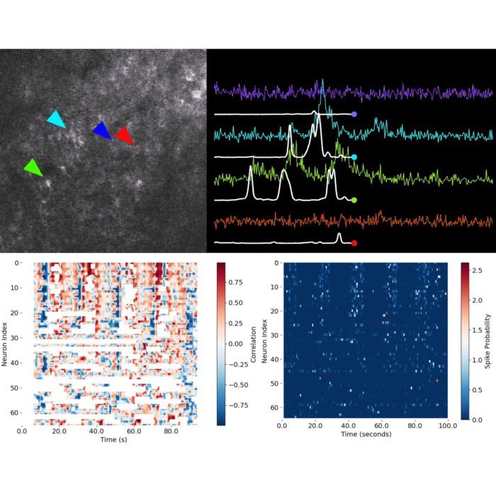
 and its spatial footprint (left).") Trace of neuron 20 (right) and its spatial footprint (left). The trace is the raw calcium signal, which is the sum of the denoised trace
Trace of neuron 20 (right) and its spatial footprint (left). The trace is the raw calcium signal, which is the sum of the denoised trace C and the residual YrA. The spatial footprint is shown as a contour plot on top of the correlation image. You can scroll through all components using the slider in the Jupyter notebook.
The plot above shows the raw traces (C+YrA) by default, but you can superimpose the denoised traces from C if you add a color to the denoised_color parameter. As always in Jupyter, if you are unsure how a method works, you can enter cnmf_refit.estimates.nb_view_components? in a new cell to get the documentation for the method.
We can also view the rejected components:
# rejected components
if len(cnmf_refit.estimates.idx_components_bad) > 0:
    cnmf_refit.estimates.nb_view_components(img=correlation_image,
                                            idx=cnmf_refit.estimates.idx_components_bad,
                                            cmap='gray',
                                            denoised_color='red')
else:
    print("No components were rejected.")
 Same plot as above, but here showing an example of a rejected component.
How to save and load results
There is a built-in save() method for the cnmf object. It can save as hdf5 or nwb:
save_path = os.path.join(Path.cwd(), 'demo_pipeline_results.hdf5')  # or add full/path/to/file.hdf5
cnmf_refit.estimates.Cn = correlation_image # squirrel away correlation image with cnmf object
cnmf_refit.save(save_path)

print(f"All results have been saved to {save_path}.")
You can use the load_CNMF() method to load your saved results. This will return a CNMF object with all the results loaded, which you can then use to access the estimates and other results:
cnmf_refit = cnmf.load_CNMF(save_path,
                            n_processes=num_processors_to_use,
                            dview=cluster)
correlation_image = cnmf_refit.estimates.Cn
print(f"Successfully loaded data.")
Post-processing
We have extracted the calcium traces C, spatial footprints A, and estimated spike counts S, which is the main goal with CNMF. But there are a few important things remaining.
Extract $\Delta F/F$ values
So far our calcium traces are in arbitrary units. It is more common to report the calcium fluorescence relative to some baseline value $F_0$:
\[\Delta F/F = (F(t)-F_0)/F_0\]Traditionally, the baseline value was calculated during some initial period of quiescence (e.g., in the visual system, when the animal was sitting in the dark). However, it is problematic to make any assumptions about a “quiet” baseline period, so researchers have started to use a moving average to calculate $F_0$. This is also what CaImAn does.
More specifically, in CaImAn the baseline is a running percentile calculated over a frames_window moving window. You can calculate $\Delta F/F$ using raw traces or the denoised traces in C (this is toggled using the use_residuals argument):
if cnmf_refit.estimates.F_dff is None:
    print('Calculating estimates.F_dff')
    cnmf_refit.estimates.detrend_df_f(quantileMin=8,
                                      frames_window=250,
                                      flag_auto=False,
                                      use_residuals=False);
else:
    print("estimates.F_dff already defined")
The estimates object will now have a F_dff field, which makes it easier to compare traces across neurons/sessions because the data is normalized. Note that F_dff values can be positive or negative because it is relative to a baseline value that is the “zero” value.
We can plot a temporal trace of a dff with time. In the following, we’ll generate a frame_time variable for plotting. This is an idealized time representation using linspace(), which assumes that images were acquired at a constant frequency throughout the session. In practice your hardware probably returns the time at which each frame was acquired, so you can use that information in your own analysis if you have it:
frame_rate = cnmf_refit.params.data['fr']
frame_pd = 1/frame_rate
frame_times = np.linspace(0, num_frames*frame_pd, num_frames)

# plot F_dff:
idx_to_plot = 30
idx_accepted = cnmf_refit.estimates.idx_components
component_number = idx_accepted[idx_to_plot]
f, ax = plt.subplots(figsize=(7,2))
ax.plot(frame_times,
        cnmf_refit.estimates.F_dff[component_number, :],
        linewidth=0.5,
        color='k');
ax.set_xlabel('Time (s)')
ax.set_ylabel('$\Delta F/F$')
ax.set_title(f"$\Delta F/F$ for unit {component_number}")
plt.tight_layout()
 Example of a $\Delta F/F$ trace for component 91. The trace is normalized to the baseline fluorescence, which is calculated as a moving percentile over the entire session. The x-axis shows time in seconds.
Select only accepted components (optional)
If you want to discard rejected components (estimates.idx_components_bad) from the estimates field, you can run select_components(). This can be useful if you are sure you only want to focus on the accepted components for downstream analysis (e.g., to share final results with colleagues, for instance).
Warning: select_components() is a destructive operation. If you run this command, the rejected components will be removed from your estimates field. If you think you might want them later, you can set the save_discarded_components parameter to True. This will let you retrieve them later with the restore_discarded_components() method.
cnmf_refit.estimates.select_components(use_object=True)
View the final refined set of remaining components:
cnmf_refit.estimates.nb_view_components(img=correlation_image,
                                        denoised_color='red',
                                        cmap='gray')
 Example $\Delta F/F$ after refining the estimates.
Visualize data, predicted activity, and residual
For our final visualization, we will use a built-in method play_movie() that shows the original movie, the predicted movie (either AC or AC + bf), and the residual.
Viewing the residuals (what the model doesn’t explain) can be extremely useful: if you end up seeing lots of neural activity in the residual movie, that means your model is leaving something important out, and you might need to go tweak some parameters. In fact, in CaImAn’s online algorithms, this is how we decide whether to add new neurons after initialization! If neural activity is discovered in the residual buffer, then it’s time to add a new neuron to AC! In the offline algorithms, it just means you might need to go check your parameters. No model is perfect: there is always some residual. You have to use your judgment about whether it is worth chasing with additional fitting.
Note: The play_movie() method has an option to include the background from the model (bf) or not (this is the include_bck Boolean parameter). If you set it to False, it will subtract bf from the original movie and will only include AC in the middle panel.
# in case you are working from loaded data, recover the raw movie
Yr, dims, num_frames = cm.load_memmap(cnmf_refit.mmap_file)
images = np.reshape(Yr.T, [num_frames] + list(dims), order='F')

# press q to quit (can take a while to start running)
cnmf_refit.estimates.play_movie(images,
                                q_max=99.9,
                                gain_res=0.5,
                                magnification=2,
                                include_bck=True,
                                use_color=True,
                                frame_range=slice(None, None, 5), # sample every 5th frame for speedup
                                thr=0); # set thr to 0.1 to see contours
 The left panel shows the original movie, the middle panel shows the predicted activity (either
 AC or AC + bf), and the right panel shows the residual (the difference between the original movie and the predicted activity). The contours of the components are overlaid on the predicted activity.
Note that if you ran select_components() to remove rejected components, the residual movie will contain activity from those rejected bits. This doesn’t mean the model is bad: the movie is simply showing false positives you already removed.
Save results to csv
When we showed how to save/load the cnmf model above, that was for working with the entire estimator object (for instance if you want to save your work and start again later). Often users just want to save certain results such as the calcium traces in C to csv and do downstream analysis later. In Python it is easiest to do this using the Pandas package.
The following shows how to save your calcium traces to a file called [IMAGE_FILE_NAME]_C_traces.csv. You can adapt this code to save other data fields such as dff. We will also save the frame times as a convenient reference:
C_trace_denoised = np.vstack((frame_times, cnmf_refit.estimates.C)).T  # Transpose so time series are in columns
C_trace_denoised_df = pd.DataFrame(C_trace_denoised)
C_trace_denoised_df.rename(columns={0:'time'}, inplace=True)
We should also save a non-denoised version of the derived Calcium traces. In the next tutorial, where we use CASCADE to infer the spike counts, we will use the non-denoised traces as input:
C_trace_raw = np.vstack((frame_times, cnmf_refit.estimates.C+cnmf_refit.estimates.YrA)).T
C_trace_raw_df = pd.DataFrame(C_trace_raw)
C_trace_raw_df.rename(columns={0:'time'}, inplace=True)
Set up file path and save using the Pandas to_csv() method:
C_trace_denoised_path = os.path.join(Path.cwd(), f'{parameters.data['fnames'][0]}_C_traces_denoised.csv')
C_trace_denoised_df.to_csv(C_trace_denoised_path, index=False)
print(f"Saved denoised estimates.C to {C_trace_denoised_path}")

C_trace_raw_path = os.path.join(Path.cwd(), f'{parameters.data['fnames'][0]}_C_traces_raw.csv')
C_trace_raw_df.to_csv(C_trace_raw_path, index=False)
print(f"Saved raw estimates.C to {C_trace_raw_path}")
Clean up open resources
We have a few resources we have left open we should take care of.
To free up processing resources, let’s shut down the cluster in case it is still open:
cm.stop_server(dview=cluster)
If you set up your logger to log to files, and you don’t want to preserve them, you can delete them with the following. If you have custom log filenames, you may have to change the log_files pattern for the following to work:
# shut down logger (otherwise will not be able to delete it)
logging.shutdown()
# delete log files:
delete_logs = True
logging_dir = cm.paths.get_tempdir()
if delete_logs:
    log_files = glob.glob(logging_dir + '\\demo_pipeline' + '*' + '.log')
    for log_file in log_files:
        print(f"Deleting {log_file}")
        os.remove(log_file)
else:
    print(f"If you want to inspect your logs they are in {logging_dir}")
print("Done with demo pipeline.")
Summary
The CaImAn toolbox offers a modern, automated approach for the analysis of calcium imaging data, which stands in contrast to traditional manual workflows, such as drawing regions of interest (ROIs) and extracting traces using Fiji’s ROI Manager. The adoption of CaImAn provides several scientific and practical advantages, but users should also be aware of certain limitations and potential pitfalls.
Advantages of CaImAn compared to manual ROI selection:
CaImAn employs advanced computational methods, such as constrained non-negative matrix factorization (CNMF) and sophisticated motion correction algorithms, to automatically detect and extract neuronal signals from large-scale imaging data. This offers several key benefits:
- Objectivity and reproducibility: Automated extraction reduces user bias and subjectivity inherent in manual selection of ROIs. The analysis is consistent across datasets and operators, enabling reproducible science.
- Scalability: CaImAn can process hundreds to thousands of neurons and large fields of view efficiently, making it suitable for modern large-scale imaging experiments, where manual annotation would be prohibitively time-consuming or impractical.
- Improved signal separation: Matrix factorization and demixing algorithms in CaImAn can resolve spatially overlapping neurons, which are difficult or impossible to separate by manual ROI drawing.
- Integrated motion correction: Robust motion correction is built into the workflow, improving the accuracy of extracted signals, especially for in vivo imaging with movement artifacts.
- Quality control and statistical filtering: CaImAn provides automated metrics to evaluate the quality of detected components, allowing for systematic exclusion of spurious or low-quality signals.
Caveats and potential pitfalls:
While CaImAn offers clear advantages, it is important to recognize its limitations:
- Parameter sensitivity: The accuracy of automatic extraction depends on careful selection of parameters (e.g., expected cell size, noise level, number of components). Suboptimal parameterization can lead to missed neurons, false positives, or poor separation.
- Algorithmic assumptions: CNMF and related algorithms make specific assumptions about signal and noise characteristics (e.g., sparseness, non-negativity, spatial contiguity) that may not fully hold in all datasets (e.g., highly dendritic or non-somatic structures).
- Black-box aspects: While automated, the internal workings of matrix factorization can be opaque; results must be critically validated (e.g., by inspecting spatial footprints and extracted traces).
- Computational requirements: Running CaImAn on large datasets requires significant computational resources (RAM, CPU), which may limit accessibility for some users.
- Learning curve: Automated workflows involve greater technical complexity and may require familiarity with Python, parameter tuning, and troubleshooting.
Despite these caveats, CaImAn represents a significant advance over manual analysis pipelines such as those implemented in Fiji. Manual ROI selection is inherently subjective, labor-intensive, and limited in its ability to separate overlapping signals or correct for motion. CaImAn, by contrast, enables scalable, objective, and statistically robust extraction of neuronal activity from complex imaging data. Users are advised to combine automated analysis with critical visual inspection and parameter validation to ensure reliable results.
Exercise 1: Modify the default CNMF parameters
Modify the CNMF relevant parameters and observe and describe what happens. You can do this by changing the params field of the cnmf_model object. For example, you can change rf, K, gSig, and merge_thr to see how it affects the results. Also use the quilt plot to visualize the effects of these changes (see section “Selecting spatial parameters”).
Exercise 2: Adapting the CaImAn pipeline to your own data
In this exercise, you will apply the CaImAn analysis pipeline to your own calcium imaging dataset. The goal is to familiarize yourself with the essential parameter adjustments required for successful data analysis and to iteratively refine your workflow based on your results.
Instructions:
- Replace the demo dataset with your own recording.
- Change the
movie_pathvariable to the file path of your calcium imaging data (or a list of file paths if your recording is split across multiple files).
- Change the
- Set data-specific parameters.
- Determine and set the appropriate frame rate (
fr) for your recording (in Hz). - Look up the decay time constant (
decay_time) for your calcium indicator (consult the manufacturer’s datasheet or recent literature). - Adjust other parameters as needed, such as spatial resolution (
dxy), neuron size (gSig), or number of components per patch (K), based on your data and experimental setup.
- Determine and set the appropriate frame rate (
- Run the full analysis pipeline as shown in the script, from motion correction through source extraction and evaluation.
- Inspect and refine your results.
- Visually inspect the extracted spatial components and calcium traces.
* If the results are not satisfactory (e.g., too many false positives/negatives, poor separation, motion artifacts), iteratively refine your parameter choices.
* Use the methods demonstrated (e.g.,
change_params(), re-running CNMF) to test new settings.
- Visually inspect the extracted spatial components and calcium traces.
* If the results are not satisfactory (e.g., too many false positives/negatives, poor separation, motion artifacts), iteratively refine your parameter choices.
* Use the methods demonstrated (e.g.,
- Save and document your final parameter choices and results.
- Save your extracted traces and spatial footprints for further analysis.
- Document which parameter settings produced the best results for your data.
Tip: If you are unsure about reasonable values for your calcium indicator, consult published reference values (e.g., GCaMP6f: decay time ~0.4 s) or ask the instructor for assistance.