Rate models as a tool for studying collective neural activity
Rate models provide simplified representations of neural activity in which the precise spike timing of individual neurons is replaced by their average firing rate. This abstraction makes it possible to study the collective behavior of large neuronal populations and to analyze network dynamics in a tractable way. I recently played around with some rate models in Python, and in this post I’d like to share what I have learned so far about their implementation and utility.
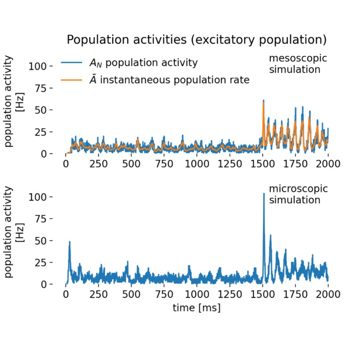
Results of a rate-model simulation (top) compared with a detailed spiking simulation (bottom). The rate model, which represents the average firing rate of a neuronal population rather than individual spikes, highlights overall dynamics and oscillatory behavior, while the spiking simulation reveals variability and single-neuron activity. In this post, we explore the implications of these differences in detail.
Introduction
Rate models emerged as a way to capture collective neural dynamics without tracking the precise timing of each spike. From a biological perspective, they are grounded in the observation that many experimental readouts (such as calcium imaging or EEG) reflect average activity of populations rather than single spike events (Dayan & Abbott, 2001). This makes rate-based descriptions particularly relevant when studying large neural systems where synchrony and fluctuations average out.
A central debate, however, is the role of rate vs. spike timing. In many brain areas, mean firing rates over tens of milliseconds correlate well with perceptual or motor variables, supporting rate coding as a useful abstraction (Gerstner et al., 2014). However, in cases where millisecond precision matters, such as auditory localization, rapid sensory transients, or precise sequence learning, spike timing conveys additional information that pure rate models cannot capture (Rieke et al., 1999). Thus, rate models are best seen as approximations valid when network activity is asynchronous and irregular, but they may fail in strongly synchronized or temporally precise regimes.
Historically, the roots of rate modeling trace back to Hebb’s postulate of cell assemblies, which emphasized average co-activity rather than individual spikes (Hebb, 1949). This inspired early mathematical formulations by Wilson and Cowan (1972), who derived coupled differential equations for interacting excitatory and inhibitory populations. These so-called cortical field models demonstrated how simple rate dynamics could produce oscillations, bistability, and other network phenomena. Since then, rate models have become a central tool in theoretical and computational neuroscience, bridging abstract neural field theories and large-scale spiking simulations.
Mathematical foundations
Spiking neuron models, such as the Hodgkin-Huxley model or the Integrate-and-Fire model, explicitly simulate the precise timing of individual spikes generated by neurons. These models capture the detailed biophysical properties of neurons and are useful for studying the dynamics of individual neurons and small networks. In contrast, rate models do not explicitly model the timing of individual spikes but instead focus on the average firing rate of the neurons. This simplification allows for more efficient simulations of large networks and provides insights into the collective behavior of neural populations, under the sacrifice of biological detail.
The primary variable in rate models is the firing rate $r(t)$, which represents the average number of spikes per unit time for a neuron or a population of neurons. The firing rate of a neuron or a neural population is typically a function of its input. This relationship can be expressed as:
\[\begin{equation} r(t) = f(I(t)) \end{equation}\]where $f$ is a non-linear function representing the neuron’s response properties, and $I(t)$ is the input current or synaptic input.
Rate models can be extended to networks where the firing rate of each neuron depends on the input from other neurons in the network. This can be described by a set of coupled differential equations:
\[\begin{equation} \tau \frac{dr_i(t)}{dt} = -r_i(t) + f\left( \sum_j w_{ij} r_j(t) + I_i(t) \right) \end{equation}\]where $\tau$ is the time constant, $w_{ij}$ is the synaptic weight from neuron $j$ to neuron $i$, and $I_i(t)$ is the external input to neuron $i$.
Population activity
Population activity $A_N$ represents the average firing rate of a group of neurons over a given time period. It provides an aggregated measure of the neuronal output by counting spikes in discrete bins and normalizing it:
\[\begin{equation} A_N(t) = \frac{1}{N \cdot \Delta t} \sum_{i=1}^{N} \sum_{k} \delta(t - t_i^k) \end{equation}\]where $N$ is the number of neurons, $\Delta t$ is the bin width, $\delta$ is the Dirac delta function, and $t_i^k$ are the spike times of neuron $i$. The fraction $1/(N \cdot \Delta t)$ normalizes the firing rate by the number of neurons and the bin width to obtain the firing rate in Hz.
Instantaneous population rates
Instantaneous population rates $\bar{A}$ represent the immediate (real-time measure) firing rate of a population, typically smoothed over a short time window to capture rapid changes in activity:
\[\begin{equation} \bar{A}(t) = \frac{\text{mean activity}}{N \cdot \Delta t} \end{equation}\]where $\text{mean activity}$ is the average firing rate recorded, e.g., by the multimeter or similar device that provides the average activity in a given time interval, $N$ is the number of neurons, and $\Delta t$ is the recording interval. The recorded mean activity is again normalized by the number of neurons and the recording interval to obtain the instantaneous firing rate in Hz.
Both, population activity $A_N$ and instantaneous population rates $\bar{A}$ are essential for characterizing the dynamics of neural populations, especially in large-scale simulations where individual neuron activities need to be aggregated and analyzed collectively. They help in identifying patterns, synchronization, oscillations, and other dynamical states in the neural network.
Types of rate models
Linear rate models
In the simplest case, the output firing rate is a linear function of the input:
\[\begin{equation} r(t) = kI(t) \end{equation}\]where $k$ is a proportionality constant. Linear models are easy to analyze but often do not capture the non-linear properties of real neurons.
Non-linear rate models
More realistic models incorporate non-linear input-output functions, such as sigmoid functions, to better represent the saturation and threshold properties of neuronal firing:
\[\begin{equation} r(t) = \frac{r_{\text{max}}}{1 + \exp(-\beta(I(t) - \theta))} \end{equation}\]where $r_{\text{max}}$ is the maximum firing rate, $\beta$ controls the steepness of the sigmoid, and $\theta$ is the threshold.
Wilson-Cowan model
This is a well-known rate model used to describe the dynamics of interacting excitatory and inhibitory populations:
\[\begin{align} \tau_E \frac{dE(t)}{dt} &= -E(t) + f_E(w_{EE}E(t) - \\ \notag & - w_{EI}I(t) + I_E(t)), \\ \tau_I \frac{dI(t)}{dt} &= -I(t) + f_I(w_{IE}E(t) - \\ \notag &- w_{II}I(t) + I_I(t)) \end{align}\]where $E(t)$ and $I(t)$ are the firing rates of the excitatory and inhibitory populations, respectively, and $w_{XY}$ are the synaptic weights between the populations.
Applications of rate models
Rate models are used to study how neural networks transition between different activity states, such as oscillations, steady states, and chaos. They help in modeling the activity of specific brain regions and understanding how different parts of the brain interact. Rate models are also used to explore how neural networks perform computations and process information.
Python simulation with NEST
NEST’s tutorial “Population rate model of generalized integrate-and-fire neurons”ꜛ provides a detailed example of simulating a population rate model using the generalized integrate-and-fire (GIF) neuron model. The tutorial replicates the main results from Schwalger et al. (2017) and is a great resource for understanding how to implement and simulate rate models in a neural simulation environment such as the NEST simulator. It uses the the effective stochastic population rate dynamics derived in Schwalger et al.’s work, which is implemented in the NEST’s gif_pop_psc_exp modelꜛ. It is applied in a Brunel network of two coupled populations, one excitatory and one inhibitory. We replicate this tutorial with some minor modifications.
We will first simulate the rate model on the so-called mesoscopic level, where the dynamics of the population activity are described by a set of ordinary differential equations (ODEs) for the average membrane potential and the average adaptation current of the populations – without simulating single neurons. In a second step, we will simulate the network on the microscopic level, where the dynamics of the individual neurons are described by the GIF model (gif_psc_expꜛ).
Mesoscopic simulation
Let’s begin with the mesoscopic simulation of the population rate model and import the necessary libraries:
import os
import matplotlib.pyplot as plt
import matplotlib.gridspec as gridspec
import numpy as np
import nest
import nest.raster_plot

# set global properties for all plots:
plt.rcParams.update({'font.size': 12})
plt.rcParams["axes.spines.top"]    = False
plt.rcParams["axes.spines.bottom"] = False
plt.rcParams["axes.spines.left"]   = False
plt.rcParams["axes.spines.right"]  = False

nest.set_verbosity("M_WARNING")
nest.ResetKernel()
nest.local_num_threads = 100
nest.rng_seed = 1
We define the following simulation parameters:
# define simulation resolutions:
dt = 0.5       # simulation resolution [ms]
dt_rec = 1.0   # resolution of the recordings [ms]
t_end = 2000.0 # simulation time [ms]

nest.resolution = dt
nest.print_time = False # set to False if the code is not executed in a Jupyter notebook or VS Code's interactive window
t0 = nest.biological_time # biological time refers to the time of the NEST kernel
Next, we define the parameters of the population rate model. We will create a population of 800 excitatory neurons and 200 inhibitory neurons. The neuronal parameters as well as the connectivity parameters are set to replicate the GIF model described in Schwalger et al. (2017)ꜛ:
# define the size of the population rate model:
size = 200
N = np.array([4, 1]) * size # number of neurons in each population; here: 800 excitatory and 200 inhibitory neurons
M = len(N)  # number of populations

# neuronal parameters:
t_ref       = 4.0 * np.ones(M)  # absolute refractory period
tau_m       = 20 * np.ones(M)   # membrane time constant
mu          = 24.0 * np.ones(M) # constant base current mu=R*(I0+Vrest)
c           = 10.0 * np.ones(M) # base rate of exponential link function
Delta_u     = 2.5 * np.ones(M)  # softness of exponential link function
V_reset     = 0.0 * np.ones(M)  # Reset potential
V_th        = 15.0 * np.ones(M) # baseline threshold (non-accumulating part)
tau_sfa_exc = [100.0, 1000.0]   # adaptation time constants of excitatory neurons
tau_sfa_inh = [100.0, 1000.0]   # adaptation time constants of inhibitory neurons
J_sfa_exc   = [1000.0, 1000.0]  # size of feedback kernel theta (= area under exponential) in mV*ms
J_sfa_inh   = [1000.0, 1000.0]  # in mV*ms
tau_theta   = np.array([tau_sfa_exc, tau_sfa_inh])
J_theta     = np.array([J_sfa_exc, J_sfa_inh])
# define connectivity parameters:
J = 0.3  # excitatory synaptic weight in mV if number of input connections is C0 (see below)
g = 5.0  # inhibition-to-excitation ratio
pconn = 0.2 * np.ones((M, M)) # connection probability
delay = 1.0 * np.ones((M, M)) # synaptic delay in ms

C0 = np.array([[800, 200], [800, 200]]) * 0.2  # constant reference matrix
C = np.vstack((N, N)) * pconn                  # numbers of input connections

# final synaptic weights scaling as 1/C:
J_syn = np.array([[J, -g * J], [J, -g * J]]) * C0 / C

taus1_ = [3.0, 6.0]  # time constants of exc./inh. postsynaptic currents (PSCs)
taus1 = np.array([taus1_ for k in range(M)])
The synaptic weights J_syn are scaled by the number of input connections C to ensure that the total input to a neuron remains constant. The applied model GIF model incorporates spike frequency adaption (SFA). This enables the neurons to adapt their firing rate in response to a constant input current. The adaptation is controlled by the adaptation time constants tau_sfa_exc and tau_sfa_inh and the feedback kernel J_theta. The model also incorporates a refractory period t_ref and a reset potential V_reset to mimic the behavior of real neurons. Postsynaptic currents (PSC) are modeled as exponential functions with time constants taus1.
We will use a step current as input to the populations to simulate the network dynamics. The step current is defined as a jump size of 20 mV in the membrane potential of the neurons at times 1500 ms and 3000 ms. The synaptic time constants for excitatory and inhibitory connections are set to 3 ms and 6 ms, respectively:
# step current input:
step = [[20.0], [20.0]]  # jump size of mu in mV
tstep = np.array([[1500.0], [1500.0]])  # times of jumps

# synaptic time constants of excitatory and inhibitory connections:
tau_ex = 3.0  # in ms
tau_in = 6.0  # in ms
Next, we create the populations,
# create the populations of GIF neurons:
nest_pops = nest.Create("gif_pop_psc_exp", M)

C_m = 250.0  # irrelevant value for membrane capacity, cancels out in simulation
g_L = C_m / tau_m

params = [
    {"C_m": C_m,
     "I_e": mu[i] * g_L[i],
     "lambda_0": c[i],  # in Hz!
     "Delta_V": Delta_u[i],
     "tau_m": tau_m[i],
     "tau_sfa": tau_theta[i],
     "q_sfa": J_theta[i] / tau_theta[i],  # [J_theta]= mV*ms -> [q_sfa]=mV
     "V_T_star": V_th[i],
     "V_reset": V_reset[i],
     "len_kernel": -1,  # -1 triggers automatic history size
     "N": N[i],
     "t_ref": t_ref[i],
     "tau_syn_ex": max([tau_ex, dt]),
     "tau_syn_in": max([tau_in, dt]),
     "E_L": 0.0}
    for i in range(M)]
nest_pops.set(params)
and further define the network connectivity:
# connect the populations:
g_syn = np.ones_like(J_syn)  # synaptic conductance
g_syn[:, 0] = C_m / tau_ex
g_syn[:, 1] = C_m / tau_in
for i in range(M):
    for j in range(M):
        nest.Connect(
            nest_pops[j],
            nest_pops[i],
            syn_spec={"weight": J_syn[i, j] * g_syn[i, j] * pconn[i, j], "delay": delay[i, j]})
To monitor the output of the network, we use a multimeter to record the mean activity of the populations and a spike recorder to record the spike times of the neurons:
# monitor the output using a multimeter (this only records with dt_rec!):
nest_mm = nest.Create("multimeter")
nest_mm.set(record_from=["n_events", "mean"], interval=dt_rec)
nest.Connect(nest_mm, nest_pops)

# monitor the output using a spike recorder:
spikerecorder = []
for i in range(M):
    spikerecorder.append(nest.Create("spike_recorder"))
    spikerecorder[i].time_in_steps = True
    nest.Connect(nest_pops[i], spikerecorder[i], syn_spec={"weight": 1.0, "delay": dt})
We set the initial value of the step current generator to zero and create the step current devices:
# set initial value (at t0+dt) of step current generator to zero:
tstep = np.hstack((dt * np.ones((M, 1)), tstep))
step  = np.hstack((np.zeros((M, 1)), step))

# create the step current devices:
nest_stepcurrent = nest.Create("step_current_generator", M)
# set the parameters for the step currents
for i in range(M):
    nest_stepcurrent[i].set(amplitude_times=tstep[i] + t0, amplitude_values=step[i] * g_L[i], origin=t0, stop=t_end)
    pop_ = nest_pops[i]
    nest.Connect(nest_stepcurrent[i], pop_, syn_spec={"weight": 1.0, "delay": dt})
Finally, we simulate the network,
# simulate the network:
t = np.arange(0.0, t_end, dt_rec)
A_N = np.ones((t.size, M)) * np.nan
Abar = np.ones_like(A_N) * np.nan
nest.Simulate(t_end + dt) # simulate 1 step longer to make sure all t are simulated:
and extract the data from the multimeter and the spike recorder for later visualization:
# extract the data from the multimeter and the spike recorder for later visualization:
data_mm = nest_mm.events
for i, nest_i in enumerate(nest_pops):
    a_i = data_mm["mean"][data_mm["senders"] == nest_i.global_id]
    a = a_i / N[i] / dt
    min_len = np.min([len(a), len(Abar)])
    Abar[:min_len, i] = a[:min_len]

    data_sr = spikerecorder[i].get("events", "times")
    data_sr = data_sr * dt - t0
    bins = np.concatenate((t, np.array([t[-1] + dt_rec])))
    A = np.histogram(data_sr, bins=bins)[0] / float(N[i]) / dt_rec
    A_N[:, i] = A
Microscopic simulation
In the microscopic simulation, we simulate the network dynamics on the level of individual neurons using the GIF model. We will create the same two populations of GIF neurons as before and connect them with the same connectivity parameters as in the mesoscopic simulation:
nest.ResetKernel()
nest.resolution = dt
nest.print_time = False
nest.local_num_threads = 1
nest.rng_seed = 1

t0 = nest.biological_time

# create the 2 populations of GIF neurons (excitatory and inhibitory):
nest_pops = []
for k in range(M):
    nest_pops.append(nest.Create("gif_psc_exp", N[k]))

# set single neuron properties:
for i in range(M):
    nest_pops[i].set(
        C_m=C_m,
        I_e=mu[i] * g_L[i],
        lambda_0=c[i],
        Delta_V=Delta_u[i],
        g_L=g_L[i],
        tau_sfa=tau_theta[i],
        q_sfa=J_theta[i] / tau_theta[i],
        V_T_star=V_th[i],
        V_reset=V_reset[i],
        t_ref=t_ref[i],
        tau_syn_ex=max([tau_ex, dt]),
        tau_syn_in=max([tau_in, dt]),
        E_L=0.0,
        V_m=0.0)

# connect the populations:
for i, nest_i in enumerate(nest_pops):
    for j, nest_j in enumerate(nest_pops):
        if np.allclose(pconn[i, j], 1.0):
            conn_spec = {"rule": "all_to_all"}
        else:
            conn_spec = {"rule": "fixed_indegree", "indegree": int(pconn[i, j] * N[j])}

        nest.Connect(nest_j, nest_i, conn_spec, syn_spec={"weight": J_syn[i, j] * g_syn[i, j], "delay": delay[i, j]})

# monitor the output using a multimeter and a spike recorder:
spikerecorder = []
for i, nest_i in enumerate(nest_pops):
    spikerecorder.append(nest.Create("spike_recorder"))
    spikerecorder[i].time_in_steps = True

    # record all spikes from population to compute population activity
    nest.Connect(nest_i, spikerecorder[i], syn_spec={"weight": 1.0, "delay": dt})

# record the membrane potential of the first Nrecord neurons of each population:
Nrecord = [5, 0]  # for each population "i" the first Nrecord[i] neurons are recorded
multimeter = []
for i, nest_i in enumerate(nest_pops):
    multimeter.append(nest.Create("multimeter"))
    multimeter[i].set(record_from=["V_m"], interval=dt_rec)
    if Nrecord[i] != 0:
        nest.Connect(multimeter[i], nest_i[: Nrecord[i]], syn_spec={"weight": 1.0, "delay": dt})

# create the step current devices and set its parameters:
nest_stepcurrent = nest.Create("step_current_generator", M)
for i in range(M):
    nest_stepcurrent[i].set(amplitude_times=tstep[i] + t0, amplitude_values=step[i] * g_L[i], origin=t0, stop=t_end)
    nest_stepcurrent[i].set(amplitude_times=tstep[i] + t0, amplitude_values=step[i] * g_L[i], origin=t0, stop=t_end)
    # optionally a stopping time may be added by: 'stop': sim_T + t0
    pop_ = nest_pops[i]
    nest.Connect(nest_stepcurrent[i], pop_, syn_spec={"weight": 1.0, "delay": dt})
# simulate 1 step longer to make sure all t are simulated
nest.Simulate(t_end + dt)
For visualization, we extract the data from the spike recorder,
# extract the data from the spike recorder:
t_micro = np.arange(0.0, t_end, dt_rec)
A_N_micro = np.ones((t.size, M)) * np.nan
for i in range(len(nest_pops)):
    data_sr = spikerecorder[i].get("events", "times") * dt - t0
    bins = np.concatenate((t_micro, np.array([t[-1] + dt_rec])))
    A = np.histogram(data_sr, bins=bins)[0] / float(N[i]) / dt_rec
    A_N_micro[:, i] = A * 1000  # in Hz
and plot the results of the mesoscopic and microscopic simulations:
# plot excitatory population:
plt.figure(1, figsize=(6, 5))
plt.subplot(2, 1, 1)
plt.plot(t, A_N[:,0] * 1000, label=f"$A_N$ population activity")
plt.plot(t, Abar[:,0] * 1000, label=f"$\\bar A$ instantaneous population rate")
plt.ylabel(f"population activity\n[Hz]")
plt.annotate(f"mesoscopic\nsimulation", xy=(0.75, 0.85), fontweight="normal",
             xycoords="axes fraction", ha="left", va="center")
plt.legend(frameon=False, loc="upper left")
plt.ylim([0, 120])
plt.yticks(np.arange(0, 101, 25))
plt.title("Population activities (excitatory population)")

plt.subplot(2, 1, 2)
plt.plot(t_micro, A_N_micro[:,0], label=f"$A_N$")
plt.ylabel(f"population activity\n[Hz]")
plt.xlabel("time [ms]")
plt.annotate(f"microscopic\nsimulation", xy=(0.75, 0.85), fontweight="normal",
             xycoords="axes fraction", ha="left", va="center")
plt.ylim([0, 120])
plt.yticks(np.arange(0, 101, 25))
plt.tight_layout()

# plot inhibitory population:
plt.figure(2, figsize=(6, 5))
plt.subplot(2, 1, 1)
plt.plot(t, A_N[:,1] * 1000, label=f"$A_N$ population activity")
plt.plot(t, Abar[:,1] * 1000, label=f"$\\bar A$ instantaneous population rate")
plt.ylabel(f"population activity\n[Hz]")
plt.annotate(f"mesoscopic\nsimulation", xy=(0.75, 0.85), fontweight="normal",
             xycoords="axes fraction", ha="left", va="center")
plt.legend(frameon=False, loc="upper left")
plt.ylim([0, 120])
plt.yticks(np.arange(0, 101, 25))
plt.title("Population activities (inhibitory population)")

# plot instantaneous population rates (in Hz):
plt.subplot(2, 1, 2)
plt.plot(t_micro, A_N_micro[:,1], label=f"$A_N$")
#plt.plot(t, A_N[:,1] * 1000, '-', alpha=0.5, label="inhibitory population")
plt.ylabel(f"population activity\n[Hz]")
plt.xlabel("time [ms]")
plt.annotate(f"microscopic\nsimulation", xy=(0.75, 0.85), fontweight="normal",
             xycoords="axes fraction", ha="left", va="center")
plt.ylim([0, 120])
plt.yticks(np.arange(0, 101, 25))
plt.tight_layout()
Results
Excitatory population
Let’s take a look at the simulation results for the excitatory population:
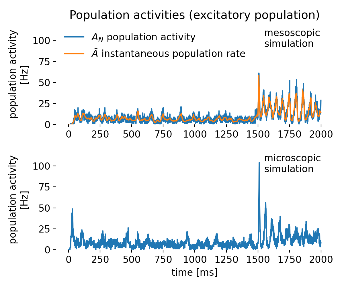 Simulated population activity of the excitatory population using mesoscopic and microscopic simulations. The top panel shows the mesoscopic activity from the rate model: $A_N$ (blue) computed from spikerecorder data as a binned histogram (discrete, noisier) and $\bar A$ (orange) from multimeter data as a continuous measure (smoother). $A_N$ is inherently noisier and strongly dependent on bin size, compared to $\bar A$, which averages activity continuously over the recording interval and therefore appears smoother. This is due to the fact that spikerecorder-based histograms capture discrete spike counts, while the multimeter integrates population firing as a continuous variable. The bottom panel shows in contrast to the rate model’s results the microscopic activity $A_N$ derived from simulated spiking GIF neurons. Mesoscopic and microscopic traces are not identical, since one averages firing rates and the other emerges from explicit spikes, but both capture the population’s strong activation after 1500 ms. Rate models thus offer efficient and smooth approximations, while spiking models preserve variability and spike-level detail.
The top panel shows the mesoscopic activity from the rate model, with $A_N$ (blue) computed from spikerecorder data as a binned histogram (discrete, noisier) and $\bar A$ (orange) from multimeter data as a continuously averaged signal (smoother). The bottom panel, in contrast, shows the microscopic activity $A_N$ derived from explicit spikes of GIF neurons. These different definitions explain why $\bar A$ appears smoother and less noisy than $A_N$, and why mesoscopic and microscopic traces are not identical.
We can clearly differentiate two distinct phases in the population activity of both panels:
1. Baseline activity (0 to 1500 ms):
In both simulations, the baseline activity of the excitatory population shows low but stable firing rates initially (0 to 1500 ms). In the mesoscopic simulation, $\bar A$ appears smoother because it is a continuous population average over the recording interval, while $A_N$ is noisier and bin-size dependent since it is based on discrete spike counts (histogram from the spikerecorder). This difference mirrors the distinct measurement definitions already noted in the figure caption.
2. Oscillatory behavior (>1500 ms):
At around 1500 ms, a step current input is applied, significantly increasing the firing rates in both simulations. The mesoscopic simulation demonstrates a rapid increase in both $A_N$ and $\bar{A}$, indicating a robust and synchronized response to the step input. The simulation reveals oscillatory behavior in both population activity and instantaneous population rate; $\bar A$ highlights the rhythmic structure more clearly due to its continuous averaging, whereas $A_N$ retains higher variance.
In the microscopic simulation, the increase in population activity is also clearly visible, but the oscillations are a bit more irregular, showing higher variability in spike counts with slightly larger amplitudes. This reflects finite-size fluctuations and the inherent stochasticity of explicit spiking dynamics. Overall, mesoscopic and microscopic traces differ in detail—one averages rates, the other arises from individual spikes—but both consistently capture the strong activation and transition to oscillatory activity after 1500 ms.
Conclusion:
The smoother and more regular patterns in the mesoscopic simulation highlight the effectiveness of rate models in capturing the overall dynamics of large neural populations. This approach reduces the computational complexity and provides clear insights into the collective behavior of neurons.
The detailed spike timing and higher variability in the microscopic simulation emphasize, on the other hand, the importance of individual neuron dynamics and interactions. This method is more computationally intensive but provides a detailed view of the neural network’s activity.
Both approaches are valuable, with rate models offering a simplified yet insightful view of population dynamics and spiking neuron models providing detailed insights into neural mechanisms.
Inhibitory population
The inhibitory population shows similar behavior as the excitatory population, but with larger $A_N$ irregularities in both the mesoscopic and microscopic simulations:
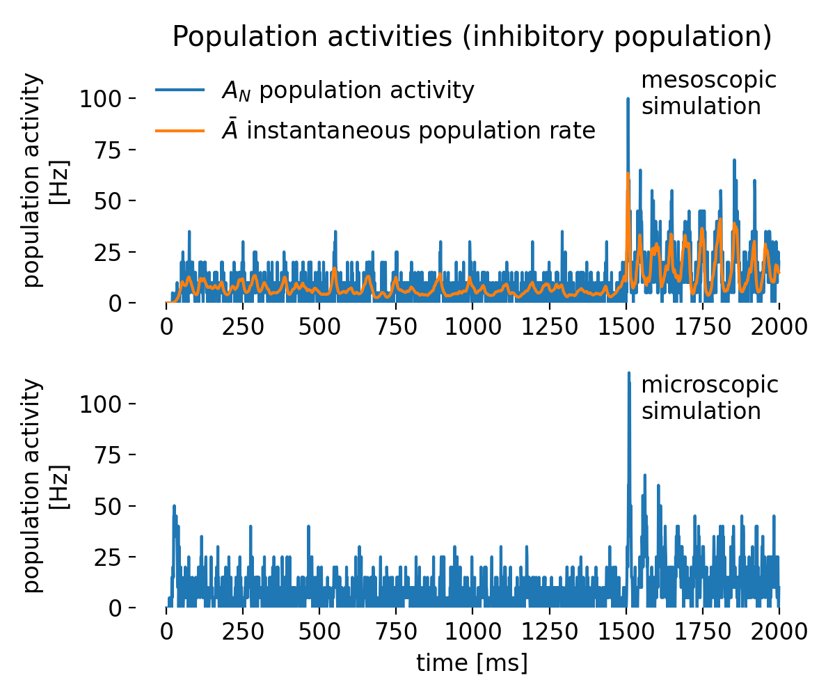 Same as above, but for the inhibitory population.
While in both simulations the population activity $A_N$ is much more noisy and showing higher amplitudes than the excitatory population, the instantaneous population rate $\bar A$ remains smooth and lets us clearly identify the oscillatory behavior in the mesoscopic simulation. Thus, the rate model is able to capture the collective dynamics of the inhibitory population effectively also in this case. As above, the difference between $A_N$ (binned, histogram-based) and $\bar A$ (continuously averaged) explains the contrast in smoothness, and microscopic traces remain more variable due to explicit spiking and finite-size effects.
Conclusion
Rate models are essential tools in computational neuroscience for studying the collective behavior of large populations of neurons. By focusing on the average firing rate of neurons, rate models provide a simplified yet insightful view of neural network dynamics. They are particularly useful for studying network-level phenomena such as oscillations, synchronization, and information processing. However, rate models sacrifice the detailed spike timing information of individual neurons, which can be crucial for understanding the underlying mechanisms of neural computation. As emphasized by Gerstner et al. (2014; there: Chapter 15ꜛ), simple rate equations may also fail to capture fast transients in population responses, which depend critically on precise spike timing. Thus, one should carefully choose between rate models and spiking neuron models based on the research question and the level of temporal detail required.
The complete code used in this blog post is available in this Github repositoryꜛ (population_rate_model.py). Feel free to modify and expand upon it, and share your insights.
References
- Wulfram Gerstner, Werner M. Kistler, Richard Naud, and Liam Paninski, Chapter 15 Fast Transients and Rate Models in Neuronal Dynamics: From Single Neurons to Networks and Models of Cognition, 2014, Cambridge University Press, ISBN: 978-1-107-06083-8, free online versionꜛ
- P. Dayan, I. F. Abbott, Theoretical Neuroscience: Computational and Mathematical Modeling of Neural Systems, 2001, MIT Press
- Donald O. Hebb, The Organization of Behavior, 1949, Wiley: New York, doi: 10.1016/s0361-9230(99)00182-3ꜛ
- F. Rieke, David Warland, Ruyter van Steveninck, & William Bialek, Spikes: Exploring the neural code, 1999, Book, MIT press, ISBN :9780262181747, urlꜛ
- Hugh R. Wilson, Jack D. Cowan, Excitatory and Inhibitory Interactions in Localized Populations of Model Neurons, 1972, Biophysical Journal, 12(1), 1–24, doi: 10.1016/S0006-3495(72)86068-5
- Wulfram Gerstner, W. M. Kistler, Spiking Neuron Models: Single Neurons, Populations, Plasticity (2002), Cambridge University Press, ISBN 0-521-81384-0, free online versionꜛ
- Schwalger, T, Deger, M, & Gerstner, W, Towards a theory of cortical columns: From spiking neurons to interacting neural populations of finite size (2017), PLoS Comput Biol, 13(4), e1005507. doi: 10.1371/journal.pcbi.1005507ꜛ
- NEST’s tutorial “Population rate model of generalized integrate-and-fire neurons”ꜛ
- NEST’s
gif_pop_psc_expmodel descriptionꜛ - NEST’s
gif_psc_expmodel descriptionꜛ

comments