Urbanczik-Senn plasticity
In 2014, Urbanczik and Sennꜛ proposed a novel learning rule for dendritic synapses in a simplified compartmental neuron model. This rule extends traditional spike-timing-dependent plasticity (STDP) by incorporating the local dendritic potential as a crucial third factor, alongside pre- and postsynaptic spike timings. In this post, we briefly introduce the Urbanczik-Senn plasticity model and discuss its implications for neural computation and learning.
 Evolution of synaptic weights according to the Urbanczik-Senn plasticity model. We will discuss them in detail in the results part.
Core concepts
Unlike traditional STDP models, which rely solely on the relative timing of pre- and postsynaptic spikes, the Urbanczik-Senn plasticity model introduces a third factor: The local dendritic potential. The neuron model therefore consists of a somatic and a dendritic compartment. The role of the somatic compartment is to integrate inputs and generate spikes, while the dendritic compartment receives synaptic inputs. The local dendritic potential $V_d(t)$ predicts the somatic activity:
\[\begin{align} C_m \frac{dV_d(t)}{dt} &= -g_L (V_d(t) - E_L) + I_d(t) \end{align}\]where $C_m$ is the membrane capacitance, $g_L$ is the somatic leak conductance, $E_L$ is the resting membrane potential, and $I_d(t)$ is the dendritic input current.
The somatic potential $V_s(t)$ is driven by the dendritic input $V_d$ and other synaptic inputs directly targeting the soma:
\[\begin{align} C_m \frac{dV_s(t)}{dt} =& -g_L (V_s(t) - E_L) + I_s(t) \\ & + g_D (V_d(t) - V_s(t)) \nonumber \end{align}\]where $I_s(t)$ is the somatic input current, and $g_D$ is the dendritic coupling conductance. The model aims to minimize the discrepancy between the somatic firing rate $\phi(U)$ and the dendritic prediction $V_d^*$ of the somatic membrane potential:
\[\begin{align} V_d^* &= \frac{g_L \cdot E_L + g_D \cdot V_d}{g_L + g_D} \end{align}\]The somatic firing rate $\phi(V_S)$ is given by:
\[\begin{align} \phi(V_S) &= \frac{\phi_{\text{max}}}{1.0 + k \cdot e^{\beta \cdot (\theta - V_S)}} \end{align}\]where $\phi_{\text{max}}$ is the maximum rate, $k$ is the rate slope, $\beta$ is a parameter controlling the steepness, and $\theta$ is the threshold potential.
Synaptic weights are adjusted based on a local dendritic prediction error, which is the difference between the actual somatic spikes and the predicted firing rate from the dendritic potential:
\[\begin{align} \Delta w_i &= \eta \cdot [S(t) - \phi(V_d^*)] \cdot \frac{\partial V_d}{\partial w_i} \end{align}\]Here, $\eta$ is the learning rate, $S(t)$ represents the somatic spike train, and $\frac{\partial V_d}{\partial w_i}$ is the contribution of synapse $i$ to the dendritic potential.
This plasticity rule is versatile and can support various learning paradigms:
- supervised learning: The somatic compartment receives a target signal that guides learning.
- unsupervised learning: The network generates its own teaching signals, promoting self-organization.
- reinforcement learning: The learning rate is modulated by a reward signal, enabling reinforcement learning.
The main advantage of this model is its ability to unify different learning paradigms under a single rule, driven by the dendritic prediction error. This rule is both biologically plausible and functionally powerful, offering a comprehensive framework for understanding and simulating synaptic plasticity in neural networks. It therefore enables more nuanced and robust learning dynamics compared to traditional STDP models:
- Predictive coding: The dendritic prediction error adjusts synaptic weights to better match somatic activity, embodying a form of predictive coding.
- Robust learning: By integrating dendritic potentials, the model captures more nuanced synaptic dynamics compared to traditional STDP, which only considers spike timings.
- Versatility: The model’s applicability to supervised, unsupervised, and reinforcement learning highlights its robustness and broad relevance to various neural processing tasks.
For further details, please refer to the original paper by Urbanczik and Senn (2014)ꜛ.
Simulation in NEST
In the following, we replicate the NEST tutorial “Weight adaptation according to the Urbanczik-Senn plasticity”ꜛ with some minor modifications. The simulation uses the pp_cond_exp_mc_urbanczik modelꜛ implemented in the NEST simulator. It consists of a two-compartment spiking point process neuron with conductance-based synapses and is capable to connect to a Urbanczik synapse urbanczik_synapseꜛ. The code reproduces the simulation results shown in figure 1B in Urbanczik’s and Senn’s original workꜛ and all simulation parameters are set accordingly except for the units: The simulation uses standard units instead of the unitless quantities used in the paper.
Let’s begin with importing the necessary libraries:
import os
import matplotlib.pyplot as plt
import matplotlib.gridspec as gridspec
import numpy as np
import nest
import nest.raster_plot
# set the verbosity of the NEST simulator:
nest.set_verbosity("M_WARNING")

# Set global properties for all plots
plt.rcParams.update({'font.size': 12})
plt.rcParams["axes.spines.top"]    = False
plt.rcParams["axes.spines.bottom"] = False
plt.rcParams["axes.spines.left"]   = False
plt.rcParams["axes.spines.right"]  = False
Next, we need to define a couple of helper functions. First, we define two functions that generate inhibitory and excitatory inputs to the soma:
# define a function for the inhibitory input:
def g_inh(amplitude, t_start, t_end):
    """
    returns weights for the spike generator that drives the inhibitory
    somatic conductance.
    """
    return lambda t: np.piecewise(t, [(t >= t_start) & (t < t_end)], [amplitude, 0.0])

# define a function for the excitatory input:
def g_exc(amplitude, freq, offset, t_start, t_end):
    """
    returns weights for the spike generator that drives the excitatory
    somatic conductance.
    """
    return lambda t: np.piecewise(
        t, [(t >= t_start) & (t < t_end)], [lambda t: amplitude * np.sin(freq * t) + offset, 0.0]
    )
Then, we define a function that calculates the matching potential $U_M$ as a function of the somatic conductances $g_E$ and $g_I$:
\[\begin{align} U_M &= \frac{g_E \cdot E_E + g_I \cdot E_I}{g_E + g_I} \end{align}\]This function computes the effective potential based on the contributions of excitatory and inhibitory synaptic inputs. It represents the equilibrium potential at the soma, considering the balance of excitatory and inhibitory inputs:
# define the matching potential:
def matching_potential(g_E, g_I, nrn_params):
    """
    returns the matching potential as a function of the somatic conductances.
    """
    E_E = nrn_params["soma"]["E_ex"]
    E_I = nrn_params["soma"]["E_in"]
    return (g_E * E_E + g_I * E_I) / (g_E + g_I)
Next, we define the dendritic prediction $V_d^*$ of the somatic membrane potential:
# define the dendritic prediction of the somatic membrane potential:
def V_w_star(V_w, nrn_params):
    """
    returns the dendritic prediction of the somatic membrane potential.
    """
    g_D = nrn_params["g_sp"]
    g_L = nrn_params["soma"]["g_L"]
    E_L = nrn_params["soma"]["E_L"]
    return (g_L * E_L + g_D * V_w) / (g_L + g_D)
We also need a function to calculate the rate function $\phi(U)$:
# define the rate function phi:
def phi(U, nrn_params):
    """
    rate function of the soma
    """
    phi_max = nrn_params["phi_max"]
    k = nrn_params["rate_slope"]
    beta = nrn_params["beta"]
    theta = nrn_params["theta"]
    return phi_max / (1.0 + k * np.exp(beta * (theta - U)))
and a function to calculate the derivative of the rate function $\phi$, i.e.,
\[\begin{align} h(V_s) &= \frac{15 \cdot \beta}{1 + \frac{e^{-\beta \cdot (\theta - V_s)}}{k}} \end{align}\]# define the derivative of the rate function phi:
def h(U, nrn_params):
"""
derivative of the rate function phi
"""
k = nrn_params["rate_slope"]
beta = nrn_params["beta"]
theta = nrn_params["theta"]
return 15.0 * beta / (1.0 + np.exp(-beta * (theta - U)) / k)
The derivative is needed to calculate the contribution of each synapse to the dendritic potential.
Now, we can start setting up the simulation. We first reset the NEST kernel and set the simulation parameters:
nest.ResetKernel()

# set simulation parameters:
n_pattern_rep     = 100  # number of repetitions of the spike pattern
pattern_duration  = 200.0
t_start           = 2.0 * pattern_duration
t_end             = n_pattern_rep * pattern_duration + t_start
simulation_time   = t_end + 2.0 * pattern_duration
n_rep_total       = int(np.around(simulation_time / pattern_duration))
resolution        = 0.1
nest.resolution   = resolution
Next, we set the neuron parameters, synapse parameters, and input parameters:
# set neuron parameters:
nrn_model = "pp_cond_exp_mc_urbanczik"
nrn_params = {
    "t_ref": 3.0,       # refractory period
    "g_sp": 600.0,      # soma-to-dendritic coupling conductance
    "soma": {
        "V_m": -70.0,   # initial value of V_m
        "C_m": 300.0,   # capacitance of membrane
        "E_L": -70.0,   # resting potential
        "g_L": 30.0,    # somatic leak conductance
        "E_ex": 0.0,    # resting potential for exc input
        "E_in": -75.0,  # resting potential for inh input
        "tau_syn_ex": 3.0,  # time constant of exc conductance
        "tau_syn_in": 3.0,  # time constant of inh conductance
    },
    "dendritic": {
        "V_m": -70.0,  # initial value of V_m
        "C_m": 300.0,  # capacitance of membrane
        "E_L": -70.0,  # resting potential
        "g_L": 30.0,   # dendritic leak conductance
        "tau_syn_ex": 3.0,  # time constant of exc input current
        "tau_syn_in": 3.0,  # time constant of inh input current
    },
    # set parameters of rate function:
    "phi_max": 0.15,    # max rate
    "rate_slope": 0.5,  # called 'k' in the paper
    "beta": 1.0 / 3.0,
    "theta": -55.0,
}
# set synapse params:
syns = nest.GetDefaults(nrn_model)["receptor_types"]
init_w = 0.3 * nrn_params["dendritic"]["C_m"]
syn_params = {
    "synapse_model": "urbanczik_synapse_wr",
    "receptor_type": syns["dendritic_exc"],
    "tau_Delta": 100.0,  # time constant of low pass filtering of the weight change
    "eta": 0.17,  # learning rate
    "weight": init_w,
    "Wmax": 4.5 * nrn_params["dendritic"]["C_m"],
    "delay": resolution,
}
# set somatic input:
ampl_exc = 0.016 * nrn_params["dendritic"]["C_m"] # amplitude of the excitatory input in nA
offset = 0.018 * nrn_params["dendritic"]["C_m"]   # offset of the excitatory input in nA
ampl_inh = 0.06 * nrn_params["dendritic"]["C_m"]  # amplitude of the inhibitory input in nA
freq = 2.0 / pattern_duration                     # frequency of the excitatory input in Hz
soma_exc_inp = g_exc(ampl_exc, 2.0 * np.pi * freq, offset, t_start, t_end) # excitatory input
soma_inh_inp = g_inh(ampl_inh, t_start, t_end)                              # inhibitory input
Then, we set the dendritic input by creating a spike pattern using Poisson generators. We record the spikes of a simulation of $n_{\text{pg}}$ Poisson generators and give the recorded spike times to spike generators:
# set dendritic input
n_pg = 200      # number of poisson generators
p_rate = 10.0  # rate in Hz
pgs = nest.Create("poisson_generator", n=n_pg, params={"rate": p_rate}) # poisson generators
prrt_nrns_pg = nest.Create("parrot_neuron", n_pg)                       # parrot neurons (for technical reasons)
nest.Connect(pgs, prrt_nrns_pg, {"rule": "one_to_one"})
spikerecorder = nest.Create("spike_recorder", n_pg)                # create the spike recorder
nest.Connect(prrt_nrns_pg, spikerecorder, {"rule": "one_to_one"})
nest.Simulate(pattern_duration)
t_srs = [ssr.get("events", "times") for ssr in spikerecorder]
After simulating the spike pattern, the spike times are stored in the variable t_srs and we need to reset the simulation kernel to start the actual simulation:
nest.ResetKernel()
nest.resolution = resolution
Now, we can create the neuron and the according spike generators:
# define neuron:
nrn = nest.Create(nrn_model, params=nrn_params) # create the Urbanczik neuron

# poisson generators are connected to parrot neurons which are connected to the mc neuron:
prrt_nrns = nest.Create("parrot_neuron", n_pg)

# create excitatory input to the soma:
spike_times_soma_inp = np.arange(resolution, simulation_time, resolution)
sg_soma_exc = nest.Create("spike_generator",
                          params={"spike_times": spike_times_soma_inp,
                                  "spike_weights": soma_exc_inp(spike_times_soma_inp)})
# create inhibitory input to the soma:
sg_soma_inh = nest.Create("spike_generator",
                          params={"spike_times": spike_times_soma_inp,
                                  "spike_weights": soma_inh_inp(spike_times_soma_inp)})

# create excitatory input to the dendrite:
sg_prox = nest.Create("spike_generator", n=n_pg)
We also create a multimeter for recording all parameters of the Urbanczik neuron, a weight recorder for recording the synaptic weights of the Urbanczik synapses, and another spike recorder for recording the spiking of the soma:
# create a multimeter for recording all parameters of the Urbanczik neuron:
rqs = nest.GetDefaults(nrn_model)["recordables"]
multimeter = nest.Create("multimeter", params={"record_from": rqs, "interval": 0.1})

# create a weight_recorder for recoding the synaptic weights of the Urbanczik synapses:
wr = nest.Create("weight_recorder")

# create another spike recorder for recording the spiking of the soma:
spikerecorder_soma = nest.Create("spike_recorder")
Finally, we connect all nodes:
# connect all nodes:
nest.Connect(sg_prox, prrt_nrns, {"rule": "one_to_one"})
nest.CopyModel("urbanczik_synapse", "urbanczik_synapse_wr", {"weight_recorder": wr[0]})
nest.Connect(prrt_nrns, nrn, syn_spec=syn_params)
nest.Connect(multimeter, nrn, syn_spec={"delay": 0.1})
nest.Connect(sg_soma_exc, nrn,
             syn_spec={"receptor_type": syns["soma_exc"],
                       "weight": 10.0 * resolution,
                       "delay": resolution})
nest.Connect(sg_soma_inh, nrn,
             syn_spec={"receptor_type": syns["soma_inh"],
                       "weight": 10.0 * resolution,
                       "delay": resolution})
nest.Connect(nrn, spikerecorder_soma)
and start the simulation, which is divided into intervals of the pattern duration:
# start the simulation, which is divided into intervals of the pattern duration:
for i in np.arange(n_rep_total):
    # Set the spike times of the pattern for each spike generator
    for sg, t_sp in zip(sg_prox, t_srs):
        nest.SetStatus(sg, {"spike_times": np.array(t_sp) + i * pattern_duration})
    nest.Simulate(pattern_duration)
After the simulation is completed, we read out the recorded data for plotting:
# read out devices for plotting:
# multimeter:
mm_events = multimeter.events
t = mm_events["times"]
V_s = mm_events["V_m.s"]
V_d = mm_events["V_m.p"]
V_d_star = V_w_star(V_d, nrn_params)
g_in = mm_events["g_in.s"]
g_ex = mm_events["g_ex.s"]
I_ex = mm_events["I_ex.p"]
I_in = mm_events["I_in.p"]
U_M = matching_potential(g_ex, g_in, nrn_params)

# weight recorder:
wr_events = wr.events
senders = wr_events["senders"]
targets = wr_events["targets"]
weights = wr_events["weights"]
times = wr_events["times"]

# spike recorder:
spike_times_soma = spikerecorder_soma.get("events", "times")
Here are the plot commands for plotting $V_s$ (membrane potential of the soma), $V_d$ (membrane potential of the dendrite), $V_d^*$ (dendritic prediction of the somatic membrane potential), $U_M$ (matching potential), somatic conductances $g_I$ and $g_E$, dendritic currents $I_{\text{in}}$ and $I_{\text{ex}}$, rates $\phi(U)$ and $\phi(V_d)$, and the rate derivative $h(V_d^*)$:
# plot the results:
lw = 1.0
fig1, (axA, axB, axC, axD, axE) = plt.subplots(5, 1, sharex=True, figsize=(8, 12))

# plot membrane potentials and matching potential:
axA.plot(t, V_s, lw=lw, label=r"$V_s$ (soma)", color="darkblue")
axA.plot(t, V_d, lw=lw, label=r"$V_d$ (dendrit)", color="deepskyblue")
axA.plot(t, V_d_star, lw=lw, label=r"$V_d^\ast$ (dendrit)", color="b", ls="--")
axA.plot(t, U_M, lw=lw, label=r"$U_M$ (soma)", color="r", ls="-", alpha=0.5)
axA.set_ylabel("membrane pot [mV]", )
axA.legend(loc="upper right")

# plot somatic conductances:
axB.plot(t, g_in, lw=lw, label=r"$g_I$", color="r")
axB.plot(t, g_ex, lw=lw, label=r"$g_E$", color="magenta")
axB.set_ylabel("somatic\nconductance [nS]")
axB.legend(loc="upper right")

# plot dendritic currents:
axC.plot(t, I_in, lw=lw, label=f"$I_$", color="r")
axC.plot(t, I_ex, lw=lw, label=f"$I_$", color="magenta")
axC.set_ylabel("dendritic\ncurrent [nA]")
axC.legend(loc="upper right")

# plot rates:
axD.plot(t, phi(V_s, nrn_params), lw=lw, label=r"$\phi(V_s)$", color="darkblue")
axD.plot(t, phi(V_d, nrn_params), lw=lw, label=r"$\phi(V_d)$", color="deepskyblue")
axD.plot(t, phi(V_d_star, nrn_params), lw=lw, label=r"$\phi(V_d^\ast)$", color="b", ls="--")
axD.plot(t, phi(V_s, nrn_params) - phi(V_d_star, nrn_params), lw=lw,
         label=r"$\phi(V_s) - \phi(V_d^\ast)$", color="r", ls="-")
axD.plot(spike_times_soma, 0.15 * np.ones(len(spike_times_soma)), ".",
         color="g", markersize=2, label="spike")
axD.legend(loc="upper right")

axE.plot(t, h(V_d_star, nrn_params), lw=lw, label=r"$h(V_d^\ast)$", color="g", ls="-")
axE.set_ylabel("rate derivative")
axE.legend(loc="upper right")
axE.set_xlim([0, 5000]) # we don't need to plot the whole simulation time

plt.tight_layout()
plt.show()
And here are the plot commands for plotting the evolution of synaptic weights:
# plot synaptic weights:
fig2, axA = plt.subplots(1, 1, figsize=(7, 4))
for i in np.arange(2, 200, 10):
    index = np.intersect1d(np.where(senders == i), np.where(targets == 1))
    if not len(index) == 0:
        axA.plot(times[index], weights[index], label="pg_{}".format(i - 2), lw=lw)

axA.set_title("Synaptic weights of Urbanczik synapses")
axA.set_xlabel("time [ms]")
axA.set_ylabel("weight")
axA.legend(fontsize=7, loc="upper right")
plt.tight_layout()
plt.show()
Results
In the following, we will take a look at the major results of the simulation, panel by panel. Note, that we limited the plots to the first 5000 ms (10000 ms for the synaptic weights) of the simulation to focus on the initial dynamics.
Membrane potentials and matching potential
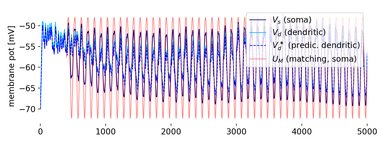
First panel: membrane potentials of the soma ($V_S$, blue) and dendrite ($V_d$, cyan), the predicted dendritic potential ($V_d^*$, dashed blue) the matching potential ($U_M$, red).
The first panel shows the membrane potentials of the soma ($V_S$, blue) and dendrite ($V_d$, cyan), the predicted dendritic potential ($V_d^*$, dashed blue), and the matching potential ($U_M$, red). Let’s describe what we see here:
- Membrane potentials ($V_s$ and $V_d$): The somatic membrane potential ($V_s$) and dendritic membrane potential ($V_d$) show oscillatory behavior. This oscillation is driven by the excitatory and inhibitory inputs defined in your simulation parameters. The somatic membrane potential oscillates around a certain value, reflecting the integration of dendritic input and other somatic inputs.
- Predicted dendritic potential ($V_d^*$): This potential is calculated based on the somatic potential and the coupling conductance between soma and dendrite. It closely follows the dendritic potential ($V_d$), indicating that the model’s prediction aligns well with the actual dendritic activity.
- Matching potential ($U_M$): This potential is derived from the somatic excitatory and inhibitory conductances. It provides a reference for the neuron’s overall excitatory and inhibitory state.
Thus, the matching potential ($U_M$) aligns with the oscillations in the somatic and dendritic potentials, indicating that the neuron is balancing its excitatory and inhibitory inputs effectively. The predicted dendritic potential ($V_d^*$) closely tracking the actual dendritic potential ($V_d$) demonstrates the accuracy of the model’s prediction mechanism. This is crucial for the learning rule, as the synaptic adjustments depend on minimizing the discrepancy between the predicted and actual potentials. The somatic firing rate, which is not directly visible in this panel but is influenced by these potentials, will be regulated based on the predicted dendritic potential, ensuring that the neuron’s output remains consistent with its input patterns.
Somatic conductances and dendritic currents
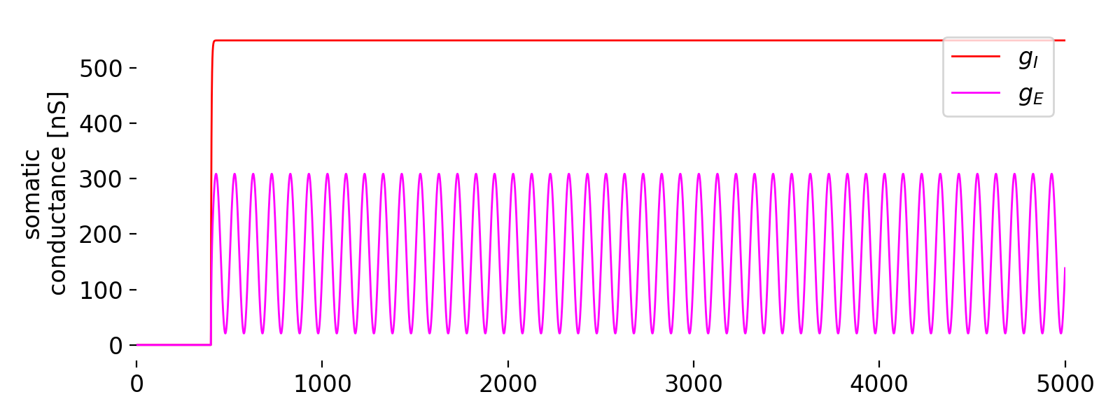
Second panel: somatic conductances ($g_I$, red and $g_E$, magenta).
The second panel shows the somatic conductances ($g_I$, red, and $g_E$, magenta). $g_I$ starts at zero and quickly rises to a constant value, indicating a steady inhibitory input throughout the simulation. The excitatory conductance $g_E$ shows a sinusoidal pattern, oscillating in sync with the sinusoidal excitatory input applied. The steady inhibitory conductance ($g_I$) serves to balance the excitatory input and control the overall excitability of the neuron. The oscillatory excitatory conductance ($g_E$) directly reflects the applied sinusoidal input, showing that the synaptic inputs are effectively driving the somatic conductances as intended.
Dendritic currents
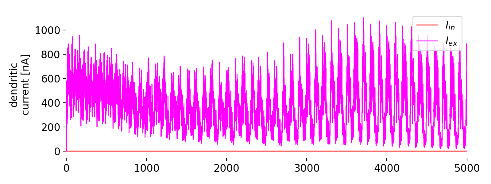
Third panel: dendritic currents ($I_{\text{in}}$, red, and $I_{\text{ex}}$, magenta).
The third panel shows the dendritic currents ($I_{\text{in}}$, red, and $I_{\text{ex}}$, magenta). The inhibitory current $I_{\text{in}}$ remains at zero, indicating that there is no inhibitory dendritic current being applied during the simulation. This is consistent with the settings used in the simulation, where only excitatory input was varied. The excitatory current $I_{\text{ex}}$ follows the sinusoidal pattern of the excitatory input, reflecting the synaptic input dynamics. The oscillatory excitatory current $I_{\text{ex}}$ oscillates with varying amplitude, showing periodic fluctuations over time. These fluctuations are influenced by the periodic excitatory input applied to the neuron, as per the settings of the simulation. This input drives the dendritic potential, which in turn affects the somatic potential and the overall activity of the neuron.
Overall, the oscillatory nature of the excitatory current reflects the sinusoidal excitatory input pattern defined in the simulation. The reduction in frequency over time may indicate a form of adaptation or a change in the neuron’s response to the input over time. The absence of inhibitory current suggests that the dynamics observed are primarily driven by excitatory inputs and their interaction with the neuron’s intrinsic properties.
Firing rates
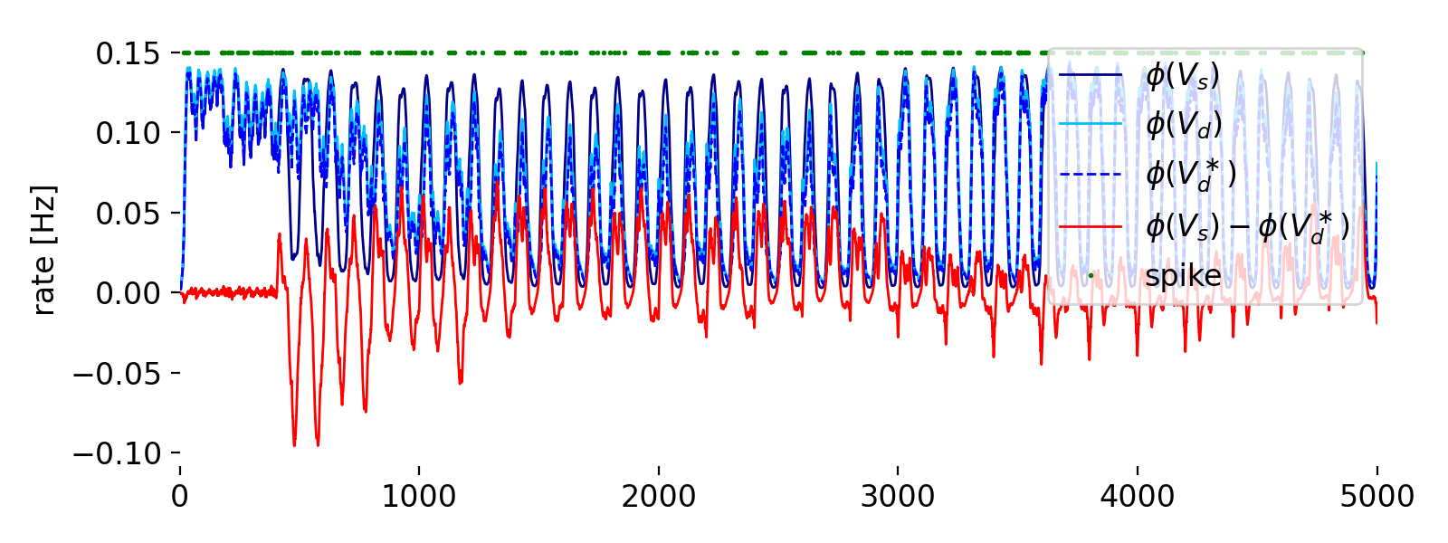
Forth panel: fireing rates $\phi(U)$ (blue), $\phi(V_d)$ (light blue), $\phi(V_d^*)$ (blue dashed), $\phi(V_S) - \phi(V_d^*)$ (red), and the spikes (green dots).
The forth panel shows the different firing rates:
- $\phi(V_s)$ (blue): The somatic firing rate calculated from the somatic membrane potential $V_s$. It oscillates due to the synaptic inputs and the intrinsic dynamics of the neuron.
- $\phi(V_d)$ (light blue): The dendritic firing rate calculated from the dendritic membrane potential $V_d$. It follows a similar oscillatory pattern to the somatic firing rate but with some differences due to the separate dynamics of the dendritic compartment.
- $\phi(V_d^*)$ (blue dashed): The predicted dendritic firing rate, calculated from the predicted dendritic potential $V_d^*$. It also oscillates and aims to match the actual dendritic firing rate.
- $\phi(V_s) - \phi(V_d^*)$ (red): The difference between the somatic firing rate and the predicted dendritic firing rate. This discrepancy drives the synaptic plasticity according to the Urbanczik-Senn learning rule. Oscillations and deviations of this line from zero highlight periods where the model adjusts the synaptic weights to minimize this error.
- Spikes (green dots): The green dots along the top axis indicate the times at which the neuron fired action potentials (spikes). These spikes occur when the somatic membrane potential crosses a certain threshold, causing the neuron to emit an action potential.
Overall, this panel illustrates the dynamic interplay between the actual somatic and dendritic firing rates, the predicted dendritic firing rate, and the resulting discrepancies that drive synaptic adjustments. The goal of the learning rule is to minimize these discrepancies over time, leading to an adaptive and predictive neural response.
Rate derivative
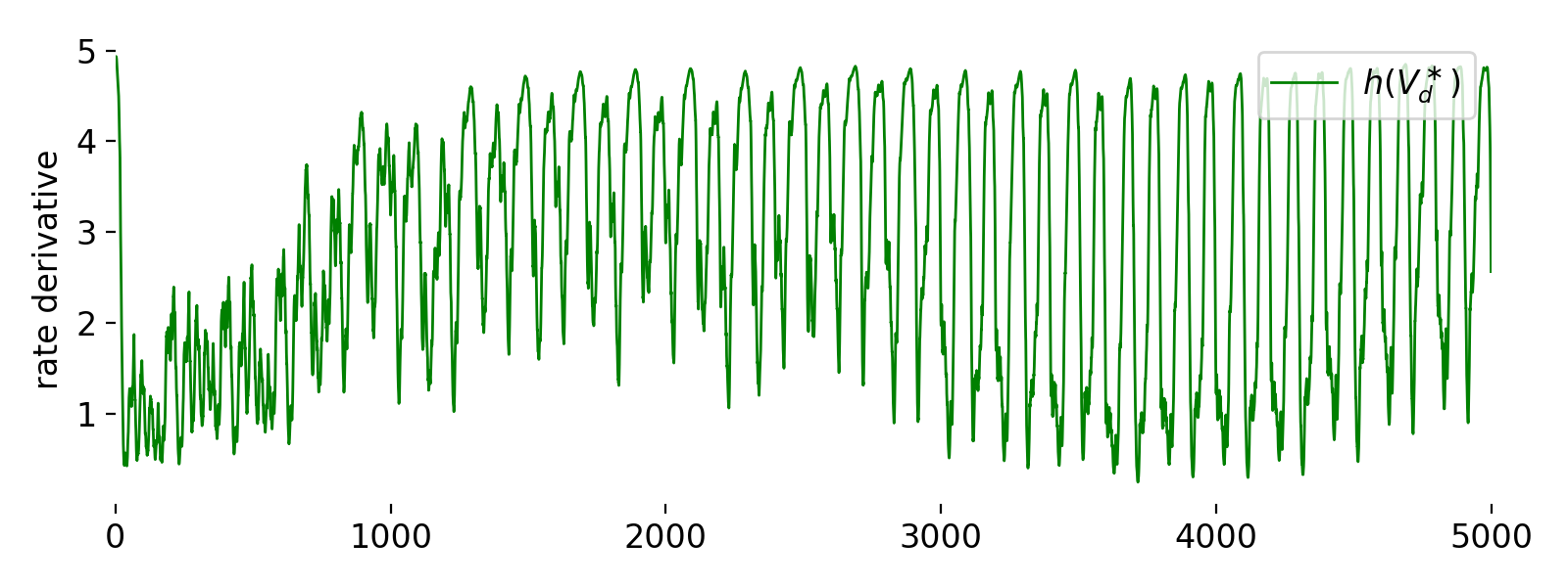
Fifth panel: rate derivative $h(V_d^*)$.
The fifth panel shows the rate derivative $h(V_d^*)$ of the rate function $\phi(V_d^*)$. Initially, $h(V_d^*)$ starts at a high value around 5, indicating a steep rate of change in the firing probability. As time progresses, the value of $h(V_d^*)$ decreases, fluctuating between 1 and 4. This fluctuation shows the dynamic adjustment of the rate derivative in response to changes in the dendritic prediction potential. The overall trend shows an increase in fluctuations, indicating that the system is responding to varying synaptic inputs and adjusting the firing rate accordingly. The initial high value could be due to the neuron adapting rapidly to the initial conditions, after which it stabilizes and responds to the ongoing synaptic inputs
This rate derivative function plays a crucial role in the learning rule, as it affects the update of synaptic weights based on the dendritic prediction error. The fluctuations in $h(V_d^*)$ indicate active learning and adaptation processes in the neuron model, as it continuously adjusts to match the predicted somatic activity with the actual somatic firing rate.
Synaptic weights
Evolutions of synaptic weights of Urbanczik synapses.
This plot shows the evolution of synaptic weights for several synapses over time. Each colored line represents the weight of a synapse from a particular parrot neuron to the Urbanczik neuron. The weights exhibit different patterns of change, with some increasing significantly while others decrease or stabilize. The diversity in weight dynamics demonstrates the model’s capacity to differentiate between inputs based on their timing and interaction with the dendritic potential, leading to a self-organized pattern of synaptic strengths.
Overall interpretation
The plots collectively illustrate the dynamics of the Urbanczik-Senn plasticity model. The membrane potentials, conductances, and currents reflect the input-driven activity of the neuron. The firing rates and their discrepancies indicate the model’s predictive coding capabilities, where the dendritic compartment predicts somatic activity. The synaptic weights evolve based on the prediction errors, demonstrating the learning rule’s impact on synaptic plasticity.
Conclusion
The Urbanczik-Senn plasticity model offers a comprehensive framework for understanding synaptic plasticity in neural networks. By integrating dendritic prediction errors, the model unifies different learning paradigms under a single rule, enabling supervised, unsupervised, and reinforcement learning. The model’s predictive coding mechanism, robust learning dynamics, and versatility make it thus a powerful tool for simulating neural processing tasks and understanding the underlying mechanisms of synaptic plasticity.
The complete code used in this blog post is available in this Github repositoryꜛ (urbanczik_senn_plasticity.py). Feel free to modify and expand upon it, and share your insights.
References
- Robert Urbanczik, Walter Senn, Learning by the dendritic prediction of somatic spiking, 2014, Neuron, Vol. 81, Issue 3, pages 521-528, doi: 10.1016/j.neuron.2013.11.030ꜛ
- NEST’s tutorial “Weight adaptation according to the Urbanczik-Senn plasticity”ꜛ
- NEST’s
pp_cond_exp_mc_urbanczikmodel descriptionꜛ - NEST’s
urbanczik_synapsesynapse descriptionꜛ


comments