Basic time series analysis

In this chapter, we learn some basic time series analysis techniques and how to read real world data from a single file and from a batch of files.

Generating a test time series

Before we start to analyse time series, we first have a look on how they are generated. We now construct a very simple time series from scratch with Python.

Create a script including the following commands:

# Create some dummy data:
import numpy as np
import matplotlib.pyplot as plt 
       # imports most relevant Matplotlib commands

# create x-values:
dx = 0.1
x_values = np.arange(0, 2*np.pi, dx)

# define parameters:
f1 = 2  # Frequency 1 in Hz
f2 = 10 # Frequency 2 in Hz
A1 = 6 # Amplitude 1
A2 = 2 # Amplitude 2

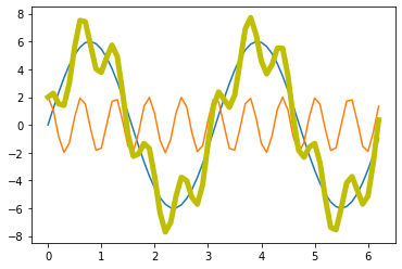
A_sin = A1 * np.sin(f1 * x_values)
A_cos = A2 * np.cos(f2 * x_values)
A_signal = A_sin + A_cos

# plots:
fig=plt.figure(1)
plt.plot(x_values, A_sin)
plt.plot(x_values, A_cos)
plt.plot(x_values, A_signal, lw=5, c="y")
plt.show()

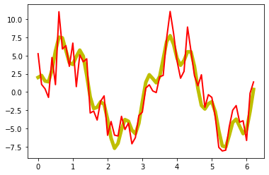
Now, we add some noise to the signal:

# add some noise:
np.random.seed(1)
A_Noise = 2
Noise = np.random.randn(len(x_values)) * A_Noise
A_signal_noisy = A_signal + Noise

fig=plt.figure(1)
plt.plot(x_values, A_signal, lw=5, c="y")
plt.plot(x_values, A_signal_noisy, lw=2, c="r")
plt.show()

Exercise 1

Basing the solution of Exercise 2 from the Data Visualization with Matplotlib chapter in the Python Basics course, copy and modify the appropriate plot commands, in order to plot

1. A_signal (add the following properties to the plot command: label="Signal", lw=2, c="pink")
2. A_signal_noisy (add the following properties to the plot command: label="Noisy signal", lw=3, c="lime")

in a single plot window. Don’t forget to annotate your plot with appropriate x- and y-labels, a title, and a legend. Also, save your plot as a PDF.

# Your solution 1 here:

Toggle solution

# Solution 1:

# Plotting:
fig = plt.figure(1)
fig.clf()

# the main plot commands:
plt.plot(x_values, A_signal,
         label="Signal", lw=2, c="pink") 
plt.plot(x_values, A_signal_noisy, 
         label="Noisy signal", lw=3, c="lime") 

# axis labels and title:
plt.xlabel("x (distance in radians)")
plt.ylabel("y")
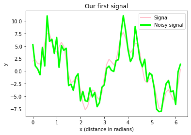
plt.title("Our first signal")

# shows a legend:
plt.legend(loc="best")

plt.show()          # finalizes the plot
fig.savefig("my_plot2.pdf", dpi=120)

The figure above includes

• our signal, which is a super-position of actually two prime signals (a sine and a cosine wave with different frequencies and amplitudes)
• our signal with some random (“background”) noise.

Signal filtering

We will now try to filter our signal in order to

1. recover the first and the second prime signal, respectively.
2. apply the same filtering operations to the noisy signal.

Let’s first aplly a so-called butter-worth filter to recover the (lower frequency) sine signal (i.e., we perform low-pass filtering). For this, we use the butter function from the scipy-filter package:

from scipy import signal # put this on top of
                         # your script

# set filter parameters:
fs = x_values.shape[0]  # Sampling frequency
fc = 5  # Cut-off frequency of the filter
w = fc / (fs / 2) # Normalize the frequency
filter_order = 10
# apply the filter function:
b, a = signal.butter(filter_order, w, 'low')

# filtering our signal
A_signal_clean = signal.filtfilt(b, a, A_signal)

plt.plot(x_values, A_signal, label='Signal', c="k")
plt.plot(x_values, A_signal_clean, label='filtered',
         c = "lime", lw=4)
plt.plot(x_values, A_sin, label='Sine', c="blue")
plt.plot(x_values, A_cos, label='Cosine', c="red")
plt.legend(loc="best")

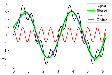
With the defined filter settings we are able to recover the sine-signal from A_signal.

In order to create a corresponding high-pass filter to also recover the high-frequency cosine signal, we would have to repeat all filter relevant commands from above. That’s actually not the way how we should do. Instead, it would be convenient if we would have our own filter-function, so that we don’t have to repeat all these complex steps.

Exercise 2: Construct a filter function

1. Recap the Function definition chapter from our Python Basics course.
2. Write a function that performs the low-pass filtering from above. Define the function in this way that the following arguments must be passed as input parameters:
   • sampling_freq for the sampling frequency,
   • cutoff_freq for the cut-off frequency of the filter,
   • filter_order for the filter order, and
   • input_signal for the input signal, that has to be processed
   • kind for the type of the filter to be applied (either low or high)
3. Apply your newly created function to A_signal, once for low-pass filtering the signal, and once for high-pass filtering it, and add corresponding plotting commands to plot
   • the unimpaired signal A_signal,
   • the high-pass filtered signal (e.g., A_clean1),
   • the low-pass filtered signal (e.g., A_clean2), and
   • a cosine and a sine wave for comparison.
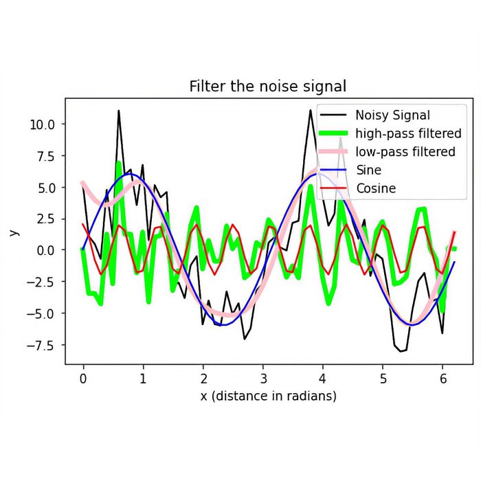
4. Apply your filter to the noisy signal A_signal_noisy, again both for low- and high-pass filtering the signal. In a new plot window, plot,
   • the noisy signal A_signal_noisy,
   • the high-pass filtered signal (e.g., A_clean1_noisy),
   • the low-pass filtered signal (e.g., A_clean2_noisy), and
   • a cosine and a sine wave for comparison. What do you notice?

# Your solution 2.2 here:

Toggle solution

# Solution 2.2:
def my_filter(sampling_freq, cutoff_freq,
              filter_order, input_signal, kind):
    """ Function for optionally high- or low-pass
        filter a given input signal
        
        sampling_freq: Sampling frequency
        cutoff_freq:   Cut-off frequency of the filter
        filter_order:  Order of the filter
        input_signal:  Signal to filter
        kind:          "high" or "low"
    """
    fc = cutoff_freq
    fs = sampling_freq
    
    w = fc / (fs / 2) # Normalize the frequency
    b, a = signal.butter(filter_order, w, kind)
    
    # filtering the signal
    filtered = signal.filtfilt(b, a, input_signal)
    
    return filtered

# Your solution 2.3 here:

Toggle solution

# Solution 2.3:
# Apply the filter function:
A_clean1=my_filter(sampling_freq = x_values.shape[0], 
               cutoff_freq = 5, filter_order = 10,
               input_signal = A_signal, kind = "high")

A_clean2=my_filter(sampling_freq = x_values.shape[0], 
               cutoff_freq = 5, filter_order = 10,
               input_signal = A_signal, kind = "low")
    
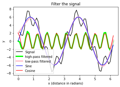
# Plotting:
fig = plt.figure(1)
fig.clf()

# the main plot commands:
plt.plot(x_values, A_signal, label='Signal', c="k")
plt.plot(x_values, A_clean1, label='high-pass filtered',
         c = "lime", lw=4)
plt.plot(x_values, A_clean2, label='low-pass filtered',
         c = "pink", lw=4)
plt.plot(x_values, A_sin, label='Sine', c="blue")
plt.plot(x_values, A_cos, label='Cosine', c="red")
plt.legend(loc="best")

# axis labels and title:
plt.xlabel("x (distance in radians)")
plt.ylabel("y")
plt.title("Filter the signal")

# shows a legend:
plt.legend(loc="best")

plt.show()          # finalizes the plot
fig.savefig("my_plot3.pdf", dpi=120)

# Your solution 2.4 here:

Toggle solution

# Solution 2.4:
A_clean1_noisy=my_filter(sampling_freq = x_values.shape[0], 
               cutoff_freq = 5, filter_order = 10,
               input_signal = A_signal_noisy, 
               kind = "high")

A_clean2_noisy=my_filter(sampling_freq = x_values.shape[0], 
               cutoff_freq = 5, filter_order = 10,
               input_signal = A_signal_noisy, 
               kind = "low")

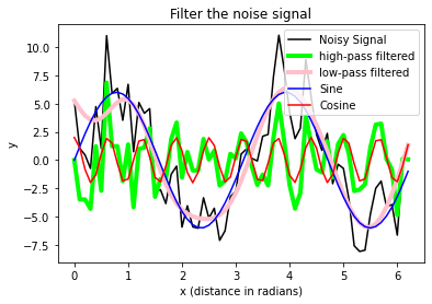
# Plotting:
fig = plt.figure(1)
fig.clf()

# the main plot commands:
plt.plot(x_values, A_signal_noisy, 
         label='Noisy Signal', c="k")
plt.plot(x_values, A_clean1_noisy, label='high-pass filtered',
         c = "lime", lw=4)
plt.plot(x_values, A_clean2_noisy, label='low-pass filtered',
         c = "pink", lw=4)
plt.plot(x_values, A_sin, label='Sine', c="blue")
plt.plot(x_values, A_cos, label='Cosine', c="red")
plt.legend(loc="best")

# axis labels and title:
plt.xlabel("x (distance in radians)")
plt.ylabel("y")
plt.title("Filter the noise signal")

# shows a legend:
plt.legend(loc="best")

plt.show()          # finalizes the plot
fig.savefig("my_plot4.pdf", dpi=120)

Advice: Matplotlib commands can grow big very quickly. It’s therefore often usefull to plug these commands into a function definition in order to keep your script readable and especially when you need to repeat your plot command(s) several times within your script.

Exercise 3: Reading real world data

1. Download the data folder “Data/Pandas_3” from the GitHub repository ꜛ (if not already done).
2. Write a script, the reads the file “mouse_1_odorA_3_results.xlsx” into a Pandas DataFrame.

3. Iterate over the keys of the DataFrame (here called df) via

   for key in df.keys():
     plt.plot(time, df[key])
   

   and plot each column of the read Excel file data into one figure. Set an appropriate titel and x- and y-labels. Use the sample frequency sampling_rate = 30.1 (unit: [1/s]) to construct the corresponding time array:

   time = np.arange(df.shape[0]) / sampling_rate
   

4. Visit the documentation website ꜛ of the scipy.signal.medfilt and read how to apply a 1D median filter to a given data array. Apply this filter to each column of the data and plot the filtered results into a new figure.

# Your solution 3.2-3.3 here:

Toggle solution

# Solution 3.2-3.3:
import pandas as pd
import os

import numpy as np
import matplotlib.pyplot as plt
from scipy import signal

# %% DEFINE PATHS
"""Define file paths:"""
file_path = "Data/Pandas_2/"
file_name = "ROI_table.xlsx"
file_1 = os.path.join(file_path, file_name)

# %% DATA READING
""" Read the Excel files with Pandas into a Pandas Dataframe:"""
#df = pd.read_excel(file_1, engine='openpyxl')
sheet_to_read = "Tabelle1"
df = pd.read_excel(file_1, index_col=0, sheet_name=sheet_to_read)
sampling_rate = 30.1
time = np.arange(df.shape[0])/sampling_rate

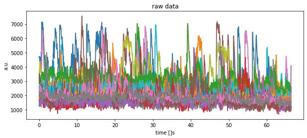
# %% SOME PLOTS
fig=plt.figure(1,figsize=(10,4))
plt.clf()
for key in df.keys():
    plt.plot(time, df[key])
plt.title("raw data")
plt.xlabel("time []s")
plt.ylabel("a.u.")
plt.show()
plt.savefig(file_1 + "raw.pdf")

# Your solution 3.4 here:

Toggle solution

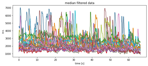
# Solution 3.4:
fig = plt.figure(2, figsize=(10, 4))
plt.clf()
for key in df.keys():
    plt.plot(time, signal.medfilt(df[key], kernel_size=9))
plt.title("median filtered data")
plt.xlabel("time [s]")
plt.ylabel("a.u.")
plt.show()
plt.savefig(file_1 + "median filtered.pdf")

df.shape

(2000, 38)

# Alternative solution:

Toggle alternative solution

# Pre-calculate (and save) median filtered data:

df_medianfiltered = np.zeros(df.shape) #This is not a DataFrame
                                       # any more, but a NUMPY
                                       # arrays

for column, key in enumerate(df.keys()):
    #print(f"column: {column}, key: {key}")
    df_medianfiltered[:, column] = \
           signal.medfilt(df[key], kernel_size=9)

fig = plt.figure(2, figsize=(10, 4))
plt.clf()
for column, key in enumerate(df.keys()):
    #df_medianfiltered[:, column] = \
    #       signal.medfilt(df[key], kernel_size=9)
    plt.plot(time, df_medianfiltered[:, column])
plt.title("median filtered data (alternative)")
plt.xlabel("time [s]")
plt.ylabel("a.u.")
plt.show()
plt.savefig(file_1 + "median filtered (alt).pdf")

Example for exporting a Pandas DataFrame into an Excel file:

# Example for exporting our processed data into a new Excel file:
df_medianfiltered_out_df = pd.DataFrame(data=df_medianfiltered)
df_medianfiltered_out_df.to_excel("data_medianfiltered.xlsx")
"""Note, for initial call of '.to_excel' you need to install
   the package/module 'xlwt' """
df_medianfiltered_out_df

	0	1	2	3	4	5	6	7	8	9	...	28	29	30	31	32	33	34	35	36	37
0	1979.681	4476.209	2814.321	2416.224	1648.606	1449.719	1744.611	2119.442	1305.099	3221.120	...	3221.120	2468.984	1750.352	1649.530	2833.220	1282.657	1231.136	3042.830	2108.877	1966.602
1	2007.620	4476.209	2838.231	2425.859	1648.606	1606.934	1886.981	2251.333	1305.119	3336.423	...	3336.423	2477.631	1854.227	1785.687	3217.644	1435.793	1374.950	3142.866	2266.636	1966.602
2	2079.598	4476.209	2866.485	2520.453	1648.606	1606.934	1938.510	2251.333	1340.275	3628.556	...	3628.556	2508.199	1875.356	1785.687	3231.953	1457.536	1374.950	3142.866	2266.829	2029.088
3	2079.598	4476.209	2946.522	2522.406	1737.614	1618.653	2003.899	2321.433	1357.278	3760.244	...	3760.244	2516.503	1875.356	1807.257	3269.945	1500.843	1425.907	3142.866	2283.250	2029.088
4	2079.598	4589.748	2948.629	2625.568	1737.614	1618.653	2086.211	2424.808	1419.689	4031.759	...	4031.759	2575.812	1875.356	1852.093	3296.585	1500.843	1500.500	3142.866	2334.456	2029.088
...	...	...	...	...	...	...	...	...	...	...	...	...	...	...	...	...	...	...	...	...	...
1995	1659.978	1988.962	2204.836	1856.755	1084.831	1065.796	1785.423	1737.096	982.970	1787.830	...	1787.830	2002.620	1782.898	1908.837	2551.720	1140.593	1198.836	1228.652	1450.763	1504.574
1996	1623.542	1988.962	2187.248	1768.047	1008.979	1058.442	1749.308	1737.096	982.970	1787.830	...	1787.830	2002.620	1760.417	1908.837	2551.720	1022.057	1198.836	1207.696	1450.763	1504.574
1997	1585.314	1981.024	2127.415	1768.047	993.758	1018.179	1749.308	1737.096	970.974	1697.901	...	1697.901	1934.899	1760.417	1908.837	2551.720	1018.071	1198.836	1193.161	1421.070	1357.963
1998	1581.983	1874.429	2110.344	1757.333	993.106	1018.179	1660.389	1737.096	957.219	1690.157	...	1690.157	1934.899	1760.417	1908.837	2546.767	1010.943	1084.129	1185.286	1421.070	1323.653
1999	1333.852	1786.643	2025.873	1757.333	936.424	1002.555	1660.389	1737.096	874.662	1658.114	...	1658.114	1934.899	1733.292	1836.423	2472.458	1010.943	962.400	1105.598	1385.715	1323.653

2000 rows × 38 columns

Grand average

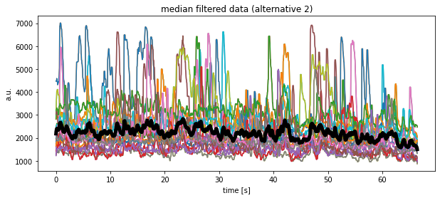
# for the sake of curiosity, let's plot the Grand Average:
fig = plt.figure(2, figsize=(10, 4))
plt.clf()
for column, key in enumerate(df.keys()):
    plt.plot(time, df_medianfiltered[:, column])
plt.plot(time, df_medianfiltered.mean(axis=1), 'k', lw=5)
plt.title("median filtered data (alternative 2)")
plt.xlabel("time [s]")
plt.ylabel("a.u.")
plt.show()
plt.savefig(file_1 + "median filtered (alt 2).pdf")

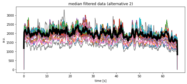
Another alternative solution would look like as follows, but at the moment I do not understand, why the medians look so different compared to the previous calculations?!

# Another alternative solution to 3.4:

Toggle another alternative solution

# Solution 3.4 (Alternative 2):
# Pre-calculate (and save) median filtered data:

df_medianfiltered_3 = signal.medfilt(df, kernel_size=9)
#This is not a DataFrame any more, but a NUMPY array

fig = plt.figure(2, figsize=(10, 4))
plt.clf()
for column in range(df_medianfiltered_3.shape[1]):
    plt.plot(time, df_medianfiltered_3[:, column])
plt.plot(time, df_medianfiltered_3.mean(axis=1), 'k', lw=5)
plt.title("median filtered data (alternative 2)")
plt.xlabel("time [s]")
plt.ylabel("a.u.")
plt.show()
plt.savefig(file_1 + "median filtered (alt 2).pdf")

Exercise 4: Apply your filter function to real world data (Exercise 3 continued)

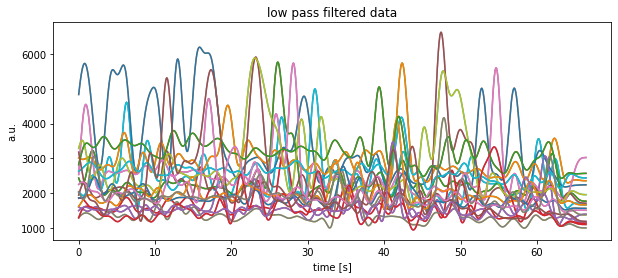
1. Apply the my_filter function, that we have written above, to the data read in Exercise 3 and plot, again, the results into a new figure.
2. Save each of your three figures (those from Exercise 3 including) into a separate PDF file.

# Your solution 4 here:

Toggle solution

# Solution 4:

# recap our previous designed filter-function:
def my_filter(sampling_freq, cutoff_freq,
              filter_order, input_signal, kind):
    """ Function for optionally high- or low-pass
        filter a given input signal

        sampling_freq: Sampling frequency
        cutoff_freq:   Cut-off frequency of the filter
        filter_order:  Order of the filter
        input_signal:  Signal to filter
        kind:          "high" or "low"
    """
    fc = cutoff_freq
    fs = sampling_freq

    w = fc / (fs / 2)  # Normalize the frequency
    b, a = signal.butter(filter_order, w, kind)

    # filtering the signal
    filtered = signal.filtfilt(b, a, input_signal)

    return filtered

fig = plt.figure(2, figsize=(10, 4))
plt.clf()
for key in df.keys():
    current_signal = my_filter(sampling_freq = sampling_rate, 
                               cutoff_freq = 0.5, 
                               filter_order = 10,
                               input_signal = df[key], 
                               kind = "low")
    plt.plot(time, current_signal)
plt.title("low pass filtered data")
plt.xlabel("time [s]")
plt.ylabel("a.u.")
plt.show()
plt.savefig(file_1 + "low-pass filtered.pdf")

Exercise 5: Batch file processing

Now, and instead of reading each Excel manually, use the following command to scan for all Excel files in the downloaded folder:

file_name = [f for f in os.listdir(file_path) if f.endswith('.xlsx')]

Copy your solutions from above into a new script. Change the new script in that way, that it iterates over all scanned file names in file_name, starting from the Pandas reading part. Play a bit around, to see, what is contained in file_name.

Hint: The automatized reading of the filenames now requires an iteration of your pipeline within a for-loop.

# Your solution 5 here:

['ROI_table.xlsx', 'ROI_table_1.xlsx', 'ROI_table_5.xlsx', 'ROI_table_4.xlsx', 'ROI_table_3.xlsx', 'ROI_table_2.xlsx']

Note that we show the result of only one Excel file here.

Toggle solution

# Solution 5 (full script):
import pandas as pd
import os
import numpy as np
import matplotlib.pyplot as plt
from scipy import signal


# %% DEFINE PATHS
"""Define file paths:"""
file_path = "Data/Pandas_2/"
file_name = [f for f in os.listdir(file_path) if f.endswith('.xlsx')]
sheet_to_read = "Tabelle1"

print(file_name)

# %% SOME FUNCTIONS
def my_filter(sampling_freq, cutoff_freq,
              filter_order, input_signal, kind):
    """ Function for optionally high- or low-pass
        filter a given input signal

        sampling_freq: Sampling frequency
        cutoff_freq:   Cut-off frequency of the filter
        filter_order:  Order of the filter
        input_signal:  Signal to filter
        kind:          "high" or "low"
    """
    fc = cutoff_freq
    fs = sampling_freq

    w = fc / (fs / 2)  # Normalize the frequency
    b, a = signal.butter(filter_order, w, kind)

    # filtering the signal
    filtered = signal.filtfilt(b, a, input_signal)

    return filtered

# %% ITERATIVELY DATA READING
""" Read the Excel files with Pandas into a Pandas Dataframe:"""
sampling_rate = 30.1 # in Hertz [1/s]

#for file in file_name:  # uncomment this line for a full run
for file in [file_name[2]]:

    # read the current Excle file:
    current_file = os.path.join(file_path, file)
    df = pd.read_excel(current_file, index_col=0, 
                       sheet_name=sheet_to_read)
    #df = pd.read_excel(current_file, engine='openpyxl')

    # calculate the current time-array:
    time = np.arange(df.shape[0]) / sampling_rate

    # plots:
    fig = plt.figure(1, figsize=(10, 4))
    plt.clf()
    for key in df.keys():
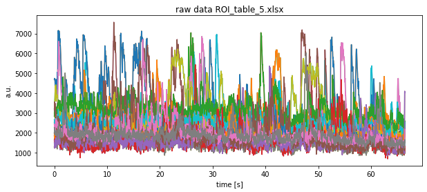
        plt.plot(time, df[key])
    plt.title(f"raw data {file}")
    plt.xlabel("time [s]")
    plt.ylabel("a.u.")
    plt.show()
    plt.savefig(file_path + file + "raw.pdf")

    fig = plt.figure(2, figsize=(10, 4))
    plt.clf()
    for key in df.keys():
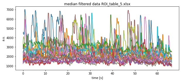
        plt.plot(time, signal.medfilt(df[key], kernel_size=9))
    plt.title(f"median filtered data {file}")
    plt.xlabel("time [s]")
    plt.ylabel("a.u.")
    plt.show()
    plt.savefig(file_path + file + "median filtered.pdf")

    fig = plt.figure(3, figsize=(10, 4))
    plt.clf()
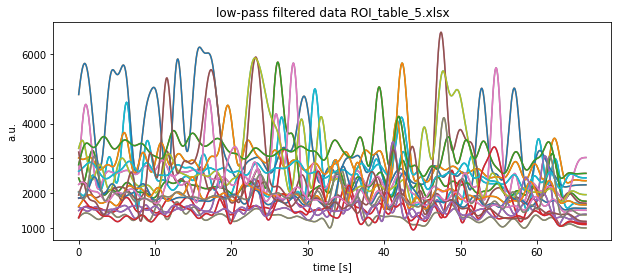
    for key in df.keys():
        current_signal = my_filter(sampling_freq=sampling_rate, 
                                   cutoff_freq=0.5, filter_order=10,
                                   input_signal=df[key], kind="low")
        plt.plot(time, current_signal)
    plt.title(f"low-pass filtered data {file}")
    plt.xlabel("time [s]")
    plt.ylabel("a.u.")
    plt.show()
    plt.savefig(file_path+file+"low pass filtered.pdf")