Adiabatic invariants and magnetic mirrors

August 18, 2020 January 23, 2026 19 minute read see also comments

Adiabatic invariants provide the central simplification behind most practical descriptions of charged particle motion in slowly varying electromagnetic fields. Besides the exact conservation laws of mechanics (energy, momentum, angular momentum under the appropriate symmetries), magnetized plasmas exhibit additional quantities that remain constant to very good approximation when field parameters vary on time scales long compared to the intrinsic periodic motions of the particle. These quantities are not “adiabatic” in the thermodynamic sense. They are adiabatic in the dynamical sense: They change only slowly compared to the characteristic periods of gyration, bounce motion, and drift. In the terrestrial magnetosphere this viewpoint turns a complicated three dimensional Lorentz trajectory into a hierarchy of nearly decoupled motions, and it explains in a quantitative way why particles can be trapped between magnetic mirror points.

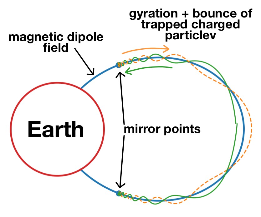
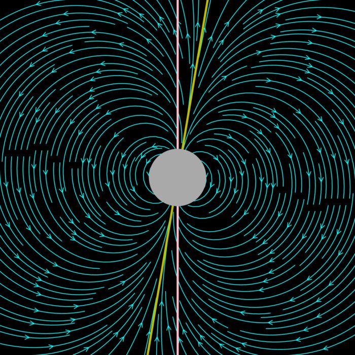
This schematic shows a magnetic mirror trajectory in an idealized Earth dipole field (2D meridional projection). The blue curve represents a single dipole field line labeled by an L shell. A positively charged particle executes fast gyromotion around the local magnetic field while its guiding center moves along the field line. As the particle travels toward higher magnetic latitude, the field strength increases; conservation of the first adiabatic invariant $\mu \propto v_\perp^2/B$ implies increasing perpendicular speed and decreasing parallel speed, until $v_\parallel=0$ at the mirror points. The particle then reverses direction and repeats this bounce motion between conjugate mirror points. Slow azimuthal drift is not shown. At the end of this post, we present a Python script with which we have simulated this trajectory numerically.

In this post, we explore the concept of adiabatic invariants in the context of charged particle motion in magnetic mirror configurations. We derive the three main adiabatic invariants and show how magnetic mirroring arises naturally from the conservation of the first invariant, the magnetic moment $\mu$.

Adiabatic invariants and the action integral

Let’s begin with the general definition of an adiabatic invariant. For a periodic degree of freedom in Hamiltonian mechanics, the action integral

\[\begin{align} J_i = \oint p_i \, dq_i \end{align}\]

is an adiabatic invariant. Here $q_i$ and $p_i$ are generalized coordinates and conjugate momenta. In plasma physics, the guiding center description of charged particle motion identifies three prominent periodic motions and, correspondingly, three adiabatic invariants:

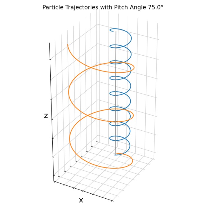
the fast gyromotion about the magnetic field line
the intermediate bounce motion along the field line between mirror points
the slow drift motion around the Earth

The ordering of time scales is essential. The first invariant is associated with the highest frequency (cyclotron motion), the second with the bounce frequency, and the third with the drift frequency.

First adiabatic invariant: The magnetic moment $\mu$

The first adiabatic invariant is the magnetic moment

\[\begin{align} \mu = \frac{1}{2}\frac{m v_\perp^2}{B} = \frac{W_\perp}{B} \end{align}\]

where $v_\perp$ is the particle velocity component perpendicular to $\mathbf{B}$ and $W_\perp$ is the corresponding perpendicular kinetic energy. In the adiabatic regime,

\[d_t \mu = 0.\]

The physical content is simple and important for everything that follows: if a particle moves into a region where $B$ is larger, conservation of $\mu$ forces $v_\perp^2$ to increase proportionally to $B$. This statement is already sufficient to understand magnetic mirroring when combined with total energy conservation, because increasing $v_\perp$ must be compensated by decreasing $v_\parallel$.

In practical guiding center models, $\mu$ is treated as an exactly conserved parameter. This is the key step that allows one to compute the parallel velocity from local field strength and initial conditions, rather than integrating the full Lorentz force at cyclotron resolution.

Second adiabatic invariant: The longitudinal invariant $J$

Consider a particle trapped between two magnetic mirror points, moving back and forth along $\mathbf{B}$. This bounce motion is periodic, hence it admits an adiabatic invariant, the longitudinal action

\[\begin{align} J = \oint m v_\parallel \, ds \end{align}\]

where $ds$ denotes an element along the magnetic field line. In this context, $J$ expresses that the integral of the parallel momentum over a full bounce period remains approximately constant when the field varies slowly compared to the bounce period.

A key magnetospheric interpretation is that even when the particle slowly drifts azimuthally around the Earth, it remains constrained to a specific field line in the idealized case. Energy conservation at the turning points (mirror points) determines the field strength at which $v_\parallel$ vanishes, but not the identity of the field line. Conservation of $J$ supplies that missing information, because it constrains the effective field line length associated with the bounce motion. Under suitable symmetry assumptions, equal length at equal field strength implies the same field line.

Third adiabatic invariant: The drift invariant $\phi$

The third adiabatic invariant is associated with the slow azimuthal drift around the Earth. In this motion the guiding center completes a periodic orbit in geomagnetic longitude. One finds that, even for slowly varying fields, the particle orbit remains on a surface enclosing the same number of magnetic field lines, meaning that the enclosed magnetic flux is approximately conserved:

\[\begin{align} \phi = \oint v_D \, r \, d\psi \end{align}\]

with $v_D$ the drift speed, $\psi$ the azimuthal angle, and $\phi$ the magnetic flux enclosed by the drift orbit. This invariant implies that the particle returns to the same geomagnetic longitude after one drift period, with the drift orbit adjusting so that $\phi$ remains (approximately) constant.

In the dipole approximation, $\phi$ is often written as

\[\begin{align} \phi = \frac{2\pi}{q^2} M \end{align}\]

where $M$ is the Earth’s dipole moment. In many practical situations this third invariant is less useful because the assumptions required for strict adiabaticity of the drift motion can break down when the field changes on time scales comparable to or shorter than the drift period.

Hierarchy of periodic motions in the Earth’s magnetosphere

The three invariants correspond to the three canonical motions:

Gyration: $\mu = \text{const.}$ for the fast cyclotron motion about $\mathbf{B}$.
Bounce motion: particles move along $\mathbf{B}$, reflect at mirror points, and repeat periodically, implying $J = \text{const.}$ on the bounce time scale.
Drift motion: particles drift around the Earth; on sufficiently long time scales the drift orbit adjusts so that $\phi = \text{const.}$ over a full azimuthal period $\psi = 2\pi$.

This ordering is frequently expressed in terms of characteristic periods: the first invariant corresponds to sub second time scales, the second to intermediate time scales (order seconds), and the third to very long time scales (order one day for typical radiation belt conditions). The exact values depend on particle energy, pitch angle, and the local field configuration, but the conceptual hierarchy is robust.

Magnetic mirroring as a consequence of $\mu$ conservation

Magnetic mirror points appear naturally once the first adiabatic invariant is combined with energy conservation. Consider a magnetostatic configuration ($\mathbf{E}=0$) in which the magnitude of the magnetic field increases along the field line toward the poles, as in the Earth’s dipole field. A charged particle with a nonzero perpendicular velocity component ($v_\perp \neq 0$) undergoes gyromotion about $\mathbf{B}$ while moving along $\mathbf{B}$ with a parallel component $v_\parallel$. In such a geometry the field lines converge toward the poles, and the particle experiences an effective force that opposes motion into regions of stronger $B$. As the particle moves poleward, $B$ increases. Conservation of $\mu$ then requires $v_\perp$ to increase. Since the total kinetic energy is conserved (for $\mathbf{E}=0$), the increase in perpendicular kinetic energy must come at the expense of parallel kinetic energy, so $v_\parallel$ decreases. The particle reaches a turning point where

\[v_\parallel = 0,\]

and is then reflected, moving back toward the equator. The turning point is the mirror point.

This is the essential mechanism behind magnetic bottles, laboratory mirrors, and the trapping of charged particles in the Earth’s magnetosphere. It also motivates a clean computational model: if one treats $\mu$ and the total speed $v$ as constants, then the parallel speed at any location can be computed algebraically from $B(\lambda)$, which is precisely the basis for the later simulation script.

Mirror force in guiding center form

A compact way to express the effect of magnetic mirroring is through the mirror force acting along the field line. In guiding center theory it takes the form

\[\begin{align} \mathbf{F}_{\mathrm{mirror}} = - \mu \, \partial_\parallel \mathbf{B} \end{align}\]

where $\partial_\parallel$ denotes the derivative along the magnetic field direction. This force points opposite the gradient of the field strength, pushing the guiding center away from regions of stronger $B$.

A full derivation can be carried out by separating $\mathbf{B}$ into components relative to a symmetry axis, linearizing $\mathbf{B}$ in the transverse direction, and averaging the Lorentz force over the fast gyromotion. For the purpose of a practical model, the key result is that the averaged parallel dynamics are governed by

\[\begin{align} m\, d_t v_\parallel = - \mu \, \frac{dB}{ds}. \end{align}\]

Here $ds$ is the arc length element along $\mathbf{B}$, and $d_t$ is the convective time derivative along the particle motion. This equation makes the physical meaning explicit: when $dB/ds>0$ in the direction of motion, the parallel velocity decreases.

Energy conservation and the turning point condition

For $\mathbf{E}=0$ the kinetic energy is conserved:

\[\begin{align} d_t\left(\frac{1}{2}m v^2\right)=0, \end{align}\]

with

\[\begin{align} v^2 = v_\perp^2 + v_\parallel^2. \end{align}\]

Using $\mu B = \tfrac{1}{2} m v_\perp^2$ from the definition of $\mu$, the total energy can be written as

\[\begin{align} \frac{1}{2}m v_\parallel^2 + \mu B = \text{const.} \end{align}\]

Differentiating this along the motion yields

\[\begin{align} d_t\left(\frac{1}{2}m v_\parallel^2\right) + \mu\, d_t B = 0. \end{align}\]

This is the compact statement of energy transfer between parallel motion and perpendicular motion in an inhomogeneous field: an increase in $B$ implies an increase in $\mu B$ and therefore a decrease in $\tfrac{1}{2}m v_\parallel^2$.

The mirror point is defined by the turning point condition

\[v_\parallel(\lambda_m)=0.\]

At that location the perpendicular speed is maximal, the pitch angle reaches $90^\circ$, and the particle reverses its motion along the field line.

Pitch angle evolution and the mirror condition

Let’s recap the pitch angle definition from our previous post on gyration, and ExB drift:

\[\begin{align} v_\perp = v\sin(\alpha), \quad v_\parallel = v\cos(\alpha). \end{align}\]

Inserting this into the magnetic moment gives

\[\begin{align} \mu = \frac{1}{2}\frac{m v^2 \sin^2(\alpha)}{B} \end{align}\]

and therefore, along a given field line,

\[\begin{align} \frac{\sin^2(\alpha_1)}{B_1} = \frac{\sin^2(\alpha_2)}{B_2}. \end{align}\]

At the mirror point, $\alpha_m = 90^\circ$, so $\sin^2(\alpha_m)=1$, which implies the practical mirror condition

\[\begin{align} \sin^2(\alpha_{eq}) = \frac{B_{eq}}{B_m}. \end{align}\]

This relation shows immediately that the mirror location depends on the equatorial pitch angle: smaller $\alpha_{eq}$ implies larger $B_m$, hence deeper penetration toward the poles, and eventually loss into the atmosphere if the mirror point lies below the top of the atmosphere. This leads naturally to the concept of the loss cone.

Dipole field model of the Earth

Near the Earth the geomagnetic field is often approximated as a dipole. In spherical coordinates $(r,\lambda)$ with magnetic latitude $\lambda$, the dipole field is

\[\begin{align} \mathbf{B} = \frac{\mu_0}{4\pi}\frac{M_E}{r^3}\left(-2\sin(\lambda)\,\hat{\mathbf{e}}_r + \cos(\lambda)\,\hat{\mathbf{e}}_\lambda\right) \end{align}\]

where $M_E$ is the Earth’s dipole moment, $r$ is the radial distance, and

\[\hat{\mathbf{e}}_r \; \text{and}\; \hat{\mathbf{e}}_\lambda\]

are unit vectors in the $r$ and $\lambda$ directions. The magnitude is

\[\begin{align} B = \frac{\mu_0}{4\pi}\frac{M_E}{r^3}\sqrt{1+3\sin^2(\lambda)}. \end{align}\]

Magnetic field lines are defined as curves tangent to $\mathbf{B}$, equivalently

\[d\mathbf{s}\times \mathbf{B}=0.\]

For an axisymmetric field, using

\[d\mathbf{s} = dr \, \hat{\mathbf{e}}_r + r \, d\lambda \, \hat{\mathbf{e}}_\lambda\]

yields

\[\frac{dr}{B_r} = \frac{r\, d\lambda}{B_\lambda}\]

and with the dipole components

\[B_r = - \frac{\mu_0}{4\pi}\frac{2M_E\sin(\lambda)}{r^3}, \quad B_\lambda = \frac{\mu_0}{4\pi}\frac{M_E\cos(\lambda)}{r^3}\]

one obtains

\[\begin{align} \frac{dr}{r} = -2\tan(\lambda)\, d\lambda. \end{align}\]

Integrating gives the dipole field line equation

\[\begin{align} r = r_{eq}\cos^2(\lambda). \end{align}\]

It is common to define the L shell parameter

\[\begin{align}L = \frac{r_{eq}}{R} \end{align}\]

where $R$ is the Earth radius. A given $L$ labels a specific field line, and typical field lines in the inner magnetosphere span approximately $L \in [1,10]$.

Using the equatorial surface field

\[\begin{align} B_E = \frac{\mu_0 M_E}{4\pi R_E^3}, \end{align}\]

the dipole field magnitude can be expressed in a convenient L shell form:

\[\begin{align} B(\lambda, L) = \frac{B_E}{L^3}\frac{\sqrt{1+3\sin^2(\lambda)}}{\cos^6(\lambda)}. \end{align}\]

This expression is exactly what a numerical guiding center mirror model needs: given $L$ and $\lambda$, it returns the local field magnitude along the chosen field line.

Loss cone and trapping condition

A particle remains trapped if its mirror points lie above the dense atmosphere. Particles with too small equatorial pitch angle mirror too deep and are lost. The set of pitch angles that lead to atmospheric loss defines the loss cone.

At the equator, the loss cone boundary $\alpha_l$ is determined by the requirement that the mirror point coincides with the Earth (or a reference altitude). In the simplified dipole treatment, one can express this through the relation

\[\begin{align} \sin^2(\alpha_l) = \frac{B_{eq}}{B_E}, \end{align}\]

and in terms of $L$ one finds

\[\begin{align} \sin^2(\alpha_l) = (4L^6 - 3L^5)^{-\frac{1}{2}}. \end{align}\]

The qualitative behavior is immediate: with increasing $L$ the field lines extend further outward, and the loss cone becomes narrower. This is why particles on high L shells can remain trapped for long times, while low L shells are more strongly affected by atmospheric loss.

Numerical simulation with Python

In the following, we simulate a magnetic mirror trajectory in an idealized dipole field using a simple guiding center model that conserves the first adiabatic invariant $\mu$. The particle’s motion along the field line is integrated using an explicit Euler scheme, while the gyromotion is represented as a small in-plane wiggle around the guiding center to visualize the gyroradius.

Before we begin, let’s clarify some assumptions and strategies. We assume:

$\mathbf{E}=0$ so that total kinetic energy is conserved.
$\mu$ is conserved (first adiabatic invariant).
motion is constrained to a fixed dipole field line labeled by $L$.

Given initial conditions at the equator (or any reference latitude) specified by $(v,\alpha_{eq})$, we will compute the constant the magnetic moment as

\[\mu = \frac{1}{2}\frac{m v^2 \sin^2(\alpha_{eq})}{B_{eq}}.\]

Then along the field line we obtain

\[v_\perp(\lambda) = \sqrt{\frac{2\mu B(\lambda)}{m}}, \quad v_\parallel(\lambda) = \pm \sqrt{v^2 - v_\perp(\lambda)^2}.\]

The mirror latitude $\lambda_m$ follows from the turning point condition $v_\parallel(\lambda_m)=0$, equivalently

\[B(\lambda_m) = \frac{B_{eq}}{\sin^2(\alpha_{eq})}.\]

Finally, to evolve the guiding center position along the field line in time we need the arc length element $ds$ along the field line. Parameterizing the field line by $\lambda$, we can write

\[\frac{d\lambda}{dt} = \frac{v_\parallel(\lambda)}{ds/d\lambda}.\]

This is the essential ordinary differential equation in our simulation: It advances the particle between mirror points. The fast gyromotion may be visualized separately by evolving a gyrophase $\phi(t)$ via

\[\frac{d\phi}{dt} = \Omega(\lambda) = \frac{q}{m}B(\lambda),\]

while keeping the guiding center constrained to the field line. This separation of motions directly reflects the adiabatic hierarchy: gyration is fast, bounce is slower, and drift is slower still.

In this way, mirror points are not imposed as an external rule but emerge as a consequence of adiabatic invariance: $\mu$ fixes how perpendicular energy scales with $B$, energy conservation converts that into a reduction of $v_\parallel$, and the turning points define the bounce motion that underlies the second invariant $J$.

Now, we implement this model in Python. Let’s begin by importing the necessary libraries and setting some plotting parameters for better aesthetics:

import numpy as np
import matplotlib.pyplot as plt
# remove spines right and top for better aesthetics
plt.rcParams['axes.spines.right'] = False
plt.rcParams['axes.spines.top'] = False
plt.rcParams['axes.spines.left'] = False
plt.rcParams['axes.spines.bottom'] = False
plt.rcParams.update({'font.size': 12})

Next, we define functions to compute the dipole field line radius and magnetic field magnitude as functions of L shell and magnetic latitude:

def r_of_lambda(L, lam):
    return L * (np.cos(lam)**2)

def dipole_Bmag(L, lam):
    c = np.cos(lam)
    s = np.sin(lam)
    return (1.0 / L**3) * np.sqrt(1.0 + 3.0*s*s) / (c**6)

and functions to compute the Cartesian coordinates along the field line, the arc length element, and the unit tangent and normal vectors:

def xyz_on_fieldline(L, lam):
    r = r_of_lambda(L, lam)
    x = r * np.cos(lam)
    z = r * np.sin(lam)
    return x, z

def ds_dlambda(L, lam):
    # Arc length along field line in meridional plane:
    # ds^2 = dr^2 + (r dθ)^2, with θ = π/2 - λ => dθ = -dλ
    r = r_of_lambda(L, lam)
    dr = -2.0 * L * np.cos(lam) * np.sin(lam)
    return np.sqrt(dr*dr + r*r)

def unit_tangent_and_normal(L, lam):
    # Numerical tangent on the field line and in-plane normal
    eps = 1e-6
    x1, z1 = xyz_on_fieldline(L, lam - eps)
    x2, z2 = xyz_on_fieldline(L, lam + eps)
    tx, tz = (x2 - x1), (z2 - z1)
    tnorm = np.sqrt(tx*tx + tz*tz) + 1e-15
    tx, tz = tx/tnorm, tz/tnorm
    nx, nz = -tz, tx
    return (tx, tz), (nx, nz)

We also need a helper function to find the mirror latitude given the equatorial pitch angle:

def find_mirror_latitude(L, alpha_eq, lam_max=1.2):
    # Condition from μ const:
    # B(λ_m) = B_eq / sin^2(alpha_eq)
    Beq = dipole_Bmag(L, 0.0)
    target = Beq / (np.sin(alpha_eq)**2)

    lams = np.linspace(0.0, lam_max, 20001)
    Bvals = dipole_Bmag(L, lams)
    idx = np.argmax(Bvals >= target)

    if Bvals[idx] < target:
        raise RuntimeError("No mirror point found: pitch angle too small or lam_max too low.")

    lam1, lam2 = lams[idx-1], lams[idx]
    B1, B2 = Bvals[idx-1], Bvals[idx]
    return lam1 + (target - B1) * (lam2 - lam1) / (B2 - B1 + 1e-15)

We then define the simulation parameters, including the L shell, equatorial pitch angle, total speed, mass, and charge:

# parameters:
L = 4.0                          # L-shell
alpha_eq = np.deg2rad(15.0)      # equatorial pitch angle; larger => mirror point closer to equator
v_total = 1.0                    # total speed (normalized)
m = 3.0
q = 300.0                       # large q/m => small gyroradius in normalized units

Next, we compute derived constants such as the equatorial magnetic field strength, initial perpendicular velocity, magnetic moment, and mirror latitude:

# derived constants (do not change!; calculates initial mu and mirror latitude):
Beq = dipole_Bmag(L, 0.0)
vperp_eq = v_total * np.sin(alpha_eq)
mu = 0.5 * m * vperp_eq**2 / Beq
lam_m = find_mirror_latitude(L, alpha_eq, lam_max=np.deg2rad(70))

# initial conditions:
lam = np.deg2rad(2.0)            # start near equator
sgn = +1.0                       # initial direction along field
phi = 0.0                        # gyro phase

and we set the time integration parameters:

# time integration:
dt = 0.002
steps = 9150 # 5000

Note that you can increase the number of steps to get a longer trajectory. However, the explicit Euler integrator which we use here is not very accurate, so for very long simulations the results may become inaccurate due to numerical errors/drift.

Next, we implement the time-stepping loop to evolve the guiding center position and gyrophase (i.e., we set-up the main simulation loop using the Euler explicit integrator):

# time-stepping loop (numerical integration):
xs, zs, dirs = [], [], []
for _ in range(steps):
    # Euler explicit integrator:
    B = dipole_Bmag(L, lam)
    vperp = np.sqrt(2.0 * mu * B / m)
    vpar = sgn * np.sqrt(max(v_total**2 - vperp**2, 0.0))

    # Guiding center evolution along the field line
    dlam_dt = vpar / (ds_dlambda(L, lam) + 1e-15)
    lam_new = lam + dt * dlam_dt

    # Gyro phase evolution
    dphi_dt = (q * B / m)
    phi_new = phi + dt * dphi_dt

    # mirror reflection at |λ| = λ_m:
    if abs(lam_new) >= lam_m:
        lam_new = np.sign(lam_new) * (2*lam_m - abs(lam_new))
        sgn *= -1.0

    # guiding center position:
    xg, zg = xyz_on_fieldline(L, lam_new)

    # Local normal direction for an in-plane "gyration wiggle"
    (_, _), (nx, nz) = unit_tangent_and_normal(L, lam_new)

    # gyroradius ρ = m v_perp / (q B):
    Bn = dipole_Bmag(L, lam_new)
    vperp_n = np.sqrt(2.0 * mu * Bn / m)
    rho = m * vperp_n / (q * Bn + 1e-15)

    # in-plane wiggle (visualization):
    x = xg + rho * np.cos(phi_new) * nx
    z = zg + rho * np.cos(phi_new) * nz

    xs.append(x)
    zs.append(z)
    dirs.append(sgn)

    lam, phi = lam_new, phi_new

xs = np.array(xs)
zs = np.array(zs)
dirs = np.array(dirs)

Before we plot the results, we calculate the field line coordinates for reference:

# calculate field line for reference for plotting:
lam_foot = np.arccos(1.0 / np.sqrt(L))          # footpoint latitude (r=1)
lam_grid = np.linspace(-lam_foot, lam_foot, 2000)
xf, zf = xyz_on_fieldline(L, lam_grid)

Finally, we create the plot showing the magnetic mirror trajectory along the dipole field line, including the mirror points and Earth representation:

fig = plt.figure(figsize=(7.85, 4.5))
# plot field line:
plt.plot(xf, zf, linewidth=2, label=f"field line (L={L:g})")
# get the indices, where the direction changes:
cuts = np.where(np.diff(dirs) != 0)[0] + 1
# define segment boundaries:
starts = np.r_[0, cuts]
ends   = np.r_[cuts, len(xs)]
# now plot each segment separately:
for s, e in zip(starts, ends):
    if dirs[s] > 0:
        plt.plot(xs[s:e], zs[s:e], linewidth=1.2, label=None,
                 c="tab:green")              # forward
    else:
        plt.plot(xs[s:e], zs[s:e], linewidth=1.2, linestyle="--", 
                 label=None, c="tab:orange")  # backward
# dummy plots for legend:
plt.plot([], [], c="tab:green", linewidth=1.2, label="forward motion")
plt.plot([], [], c="tab:orange", linewidth=1.2, linestyle="--", label="backward motion")

# earth:
theta = np.linspace(0, 2*np.pi, 600)
plt.plot(np.cos(theta), np.sin(theta), linewidth=2, label="Earth",
         c="tab:red")

# mirror points:
xM, zM = xyz_on_fieldline(L, lam_m)
plt.scatter([xM, xM], [zM, -zM], s=35, label="mirror points")

plt.gca().set_aspect("equal", adjustable="box")
plt.xlabel("x ($R_E$)")
plt.ylabel("z ($R_E$)")
plt.title("Magnetic mirror motion on a dipole field line (2D projection)\nAdiabatic model with μ const and energy const\n")
plt.legend(loc="upper right", bbox_to_anchor=(1.50, 1.0))
plt.xlim(-1.1, L*1.1)
plt.ylim(-2, 2)

# set x and y ticks:
plt.xticks(np.arange(-1, L+1, 1))
plt.yticks(np.arange(-2, 2.5, 1))

plt.tight_layout()

out_path = f"magnetic_mirror_2d_L{L}_alpha{np.rad2deg(alpha_eq):.1f}deg.png"
plt.savefig(out_path, dpi=200)
#plt.close(fig)

rho_eq = m * vperp_eq / (q * Beq)
print(f"mirror latitude λ_m = {np.rad2deg(lam_m):.2f} deg")
print(f"equatorial gyroradius ρ_eq ≈ {rho_eq:.3f} R_E")

The resulting plot looks as follows:

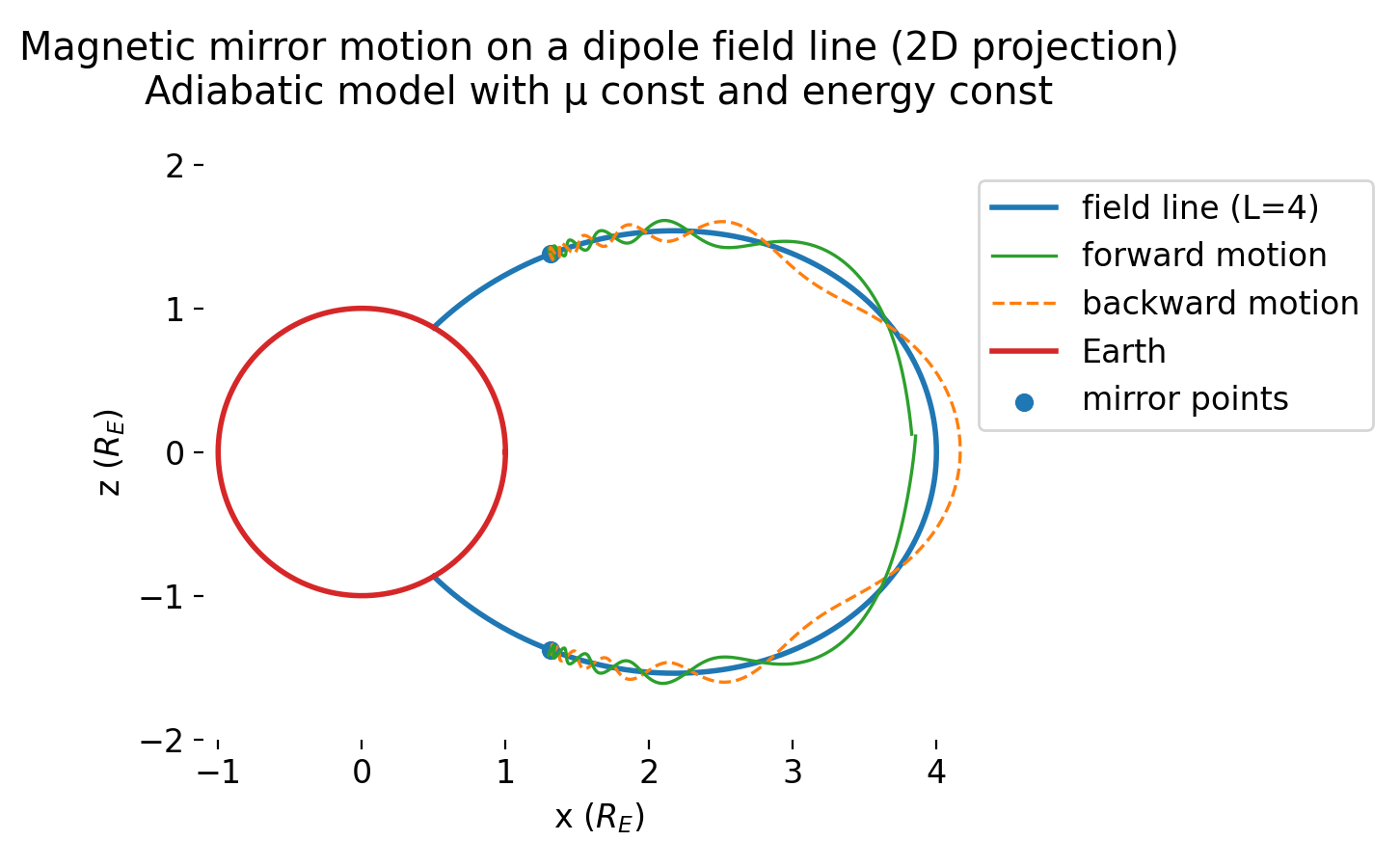
The plot shows the numerically simulated magnetic mirror motion of a positively charged particle on a dipole magnetic field line in a 2D meridional projection. The blue curve represents a single dipole field line labeled by $L=4$. The particle’s guiding center moves along this field line while executing a fast gyromotion, visualized as a small in-plane oscillation around the guiding center. As the particle propagates toward higher magnetic latitude, the magnetic field strength increases and conservation of the first adiabatic invariant $\mu$ forces an increase in perpendicular velocity at the expense of the parallel component. At the mirror points (blue markers), the parallel velocity vanishes and the particle reverses direction, producing a periodic bounce motion between conjugate hemispheres. Forward and backward segments of the bounce motion are shown separately. The Earth is drawn for scale. Slow azimuthal drift is not included in this 2D projection.

The simulation reproduces the essential features of magnetic trapping in an idealized dipole field using only adiabatic invariance and energy conservation. Mirror points arise naturally from the dynamics rather than being imposed externally: once the magnetic moment $\mu$ is fixed by the equatorial pitch angle, the local field strength uniquely determines the partition of kinetic energy between perpendicular and parallel motion. As the particle moves into regions of stronger magnetic field, the parallel velocity decreases until it vanishes, defining the turning points of the bounce motion.

The guiding center trajectory follows a single dipole field line throughout the simulation, reflecting the assumed conservation of the second adiabatic invariant on bounce time scales. The small oscillatory deviation from the field line represents the gyromotion and is included only for visualization; in reality, the true gyration occurs in the plane perpendicular to the local magnetic field and cannot be represented exactly in a single meridional plane. The slight phase mismatch observed after many bounce periods is a numerical artifact of the explicit Euler integration scheme, as noted above, and does not reflect physical diffusion or violation of adiabatic invariance. A higher-order or symplectic integrator would reduce this drift without changing the qualitative behavior.

Overall, the model demonstrates how magnetic mirroring and bounce motion follow directly from the first adiabatic invariant, providing a transparent bridge between analytical theory and numerical experimentation.

Update and code availability: This post and its accompanying Python code were originally drafted in 2020 and archived during the migration of this website to Jekyll and Markdown. In January 2026, I substantially revised and extended the code. The updated and cleaned-up implementation is now available in this new GitHub repositoryꜛ. Please feel free to experiment with it and to share any feedback or suggestions for further improvements.

References and further reading

Wolfgang Baumjohann and Rudolf A. Treumann, Basic Space Plasma Physics, 1997, Imperial College Press, ISBN: 1-86094-079-X
J. A. Bittencourt, Fundamentals of Plasma Physics, 2004, Springer, ISBN: 978-0-387-20975-3