Magnetic reconnection via X-point collapse
In our previous post, we introduced a toy model where magnetic reconnection was illustrated using a Harris-type current sheet driven by a localized inflow–outflow pattern and a spatially localized resistivity. That setup was deliberately chosen to mirror the canonical Sweet–Parker cartoon: anti-parallel magnetic fields, inflow from above and below, a confined diffusion region, and horizontal exhausts.
In this post, we explore a complementary toy model of magnetic reconnection based on the collapse of an X-point under a prescribed stagnation flow. This model highlights how different geometries and driving conditions can shape reconnection dynamics, while still governed by the same underlying resistive induction physics.
Here, a closely related but conceptually distinct toy model is considered. While it is governed by the same underlying induction physics, its geometry, boundary conditions, and driving emphasize a different reconnection scenario: the collapse of an X-point under a prescribed stagnation flow.
Governing equations
As before, the magnetic field is represented in two dimensions through an out-of-plane vector potential $A(x,y,t)$, such that
\[B_x = \frac{\partial A}{\partial y}, \quad B_y = -\frac{\partial A}{\partial x}.\]The time evolution of $A$ follows a kinematic, resistive induction equation,
\[\frac{\partial A}{\partial t} + \mathbf{v}\cdot\nabla A = \eta \nabla^2 A.\]The flow field $\mathbf{v}(x,y)$ is prescribed and does not respond to the magnetic field. There is no momentum equation, no pressure, no energy balance, and no self-consistent force coupling. As in the main post, this is therefore not a full MHD simulation, but a reduced model designed to isolate the interplay between advection, diffusion, and magnetic topology.
In both models, reconnection is enabled solely by the resistive term. In the ideal limit ($\eta \to 0$), the magnetic flux function is frozen into the flow, and the topology of the field lines would remain unchanged.
Initial magnetic configuration: X-point vs. current sheet
The most fundamental difference lies in the initial magnetic geometry. In this follow-up model, the starting point is an X-type magnetic field,
\[A_{\mathrm{X}}(x,y) = B_0 x y,\]which already contains a hyperbolic null point at the origin. A localized perturbation is added to sharpen gradients near the center and promote the formation of a thin current layer, but the separatrix structure is present from the outset.
By contrast, the model used in the previous post begins from a Harris-type current sheet, corresponding to anti-parallel magnetic fields across a planar layer. In that case, the X-point topology emerges dynamically as a consequence of the perturbation and resistive evolution.
Physically, both configurations are standard idealizations in reconnection theory. The Harris sheet emphasizes reconnection as a process occurring in an extended current layer, whereas the X-point setup emphasizes the collapse and distortion of an existing magnetic null.
Prescribed flow: Global stagnation vs. localized driving
A second key difference is the flow field. In this model, the velocity is taken to be a global incompressible stagnation flow,
\[\mathbf{v}(x,y) = (-\alpha x, +\alpha y),\]which compresses the magnetic field toward the origin in one direction while stretching it in the orthogonal direction. This type of flow is a classical driver of X-point collapse: advection sharpens gradients near the null, increasing the current density until resistive diffusion becomes important.
In the previous model, the stagnation flow is instead localized by an exponential envelope. This confines the driving to a finite region around the reconnection site and leaves the outer domain largely undisturbed. The localized flow better matches the usual pedagogical picture of plasma inflow toward a narrow diffusion region embedded in an otherwise quiescent environment.
The global nature of the flow in the present model means that the entire domain participates in the deformation. This makes the system more sensitive to boundary conditions and leads to large-scale field line distortion that is absent in the localized-flow setup.
Resistivity and boundary conditions
The resistivity ($\eta$) in this follow-up model is taken to be spatially uniform. Diffusion therefore acts everywhere, not just in a narrowly defined diffusion region. Over time, this leads to a global smoothing of the magnetic flux function once strong gradients have developed.
In contrast, the previous model introduces a localized enhancement of resistivity on top of a weak background. That choice enforces a clear conceptual separation between ideal inflow regions and a non-ideal diffusion region, closely following standard reconnection cartoons.
Boundary conditions also differ. Here, periodic boundaries are used in both spatial directions. This choice is mathematically convenient and common in idealized studies of X-point collapse, but it implies that inflow and outflow regions are topologically connected across the domain boundaries. In the Harris-sheet model, periodicity is retained only along the current sheet, while Neumann conditions are applied across it, yielding a geometry that more naturally represents inflow from “above” and “below.”
Python code
We begin again by importing the necessary libraries:
from __future__ import annotations

import os
from pathlib import Path

import numpy as np
import matplotlib.pyplot as plt
import imageio.v2 as imageio
We then define utility functions for:
- ensuring output directories exist,
- computing spatial derivatives with periodic boundary conditions,
- initializing the magnetic flux function with an X-point and perturbation, and
- computing the magnetic field components and current density proxy from the flux function.
# function to ensure output directory exists:
def ensure_dir(p: str | Path) -> None:
    Path(p).mkdir(parents=True, exist_ok=True)

# central difference and Laplacian with periodic BC:
def ddx_central(f: np.ndarray, dx: float) -> np.ndarray:
    """Central difference with periodic BC in x."""
    return (np.roll(f, -1, axis=1) - np.roll(f, 1, axis=1)) / (2.0 * dx)

# central difference and Laplacian with periodic BC:
def ddy_central(f: np.ndarray, dy: float) -> np.ndarray:
    """Central difference with periodic BC in y."""
    return (np.roll(f, -1, axis=0) - np.roll(f, 1, axis=0)) / (2.0 * dy)

# Laplacian with periodic BC:
def laplacian_periodic(f: np.ndarray, dx: float, dy: float) -> np.ndarray:
    """2D Laplacian with periodic BC in both directions."""
    f_xx = (np.roll(f, -1, axis=1) - 2.0 * f + np.roll(f, 1, axis=1)) / (dx * dx)
    f_yy = (np.roll(f, -1, axis=0) - 2.0 * f + np.roll(f, 1, axis=0)) / (dy * dy)
    return f_xx + f_yy

# initial condition for A(x,y):
def make_initial_A(X: np.ndarray, Y: np.ndarray,
                   B0: float = 1.0,
                   a: float = 0.15,
                   sheet_sigma: float = 0.12,
                   mode: int = 1) -> np.ndarray:
    """
    X-point flux plus a perturbation that seeds a thin current sheet around x=0.

    A_X = B0 * x * y  gives an X-type field.
    The perturbation adds strong gradients near x=0, supporting a current layer.
    """
    A_x = B0 * X * Y
    A_pert = a * np.cos(2.0 * np.pi * mode * Y) * np.exp(-(X * X) / (2.0 * sheet_sigma * sheet_sigma))
    return A_x + A_pert

# compute B and Jz from A:
def compute_fields(A: np.ndarray, dx: float, dy: float) -> tuple[np.ndarray, np.ndarray, np.ndarray]:
    """Return Bx, By, and current proxy Jz = -∇²A."""
    Bx = ddy_central(A, dy)
    By = -ddx_central(A, dx)
    Jz = -laplacian_periodic(A, dx, dy)
    return Bx, By, Jz
Next, we define the main plotting function to visualize the magnetic flux contours, current density magnitude, and magnetic field vectors at each time step:
def plot_frame(A: np.ndarray,
               X: np.ndarray,
               Y: np.ndarray,
               dx: float,
               dy: float,
               t: float,
               out_png: str,
               quiver_stride: int = 10,
               n_contours: int = 28) -> None:
    Bx, By, Jz = compute_fields(A, dx, dy)

    Jabs = np.abs(Jz)
    Jmax = np.percentile(Jabs, 99.5) + 1e-12

    fig = plt.figure(figsize=(8.0, 6.5), dpi=140)
    ax = fig.add_subplot(1, 1, 1)

    im = ax.imshow(
        Jabs,
        origin="lower",
        extent=[X.min(), X.max(), Y.min(), Y.max()],
        interpolation="bilinear",
        aspect="auto",
        vmin=0.0,
        vmax=Jmax)
    cb = fig.colorbar(im, ax=ax, shrink=0.9)
    cb.set_label(r"$|J_z| \propto |\nabla^2 A|$ (arb.)")

    levels = np.linspace(np.percentile(A, 2), np.percentile(A, 98), n_contours)
    ax.contour(X, Y, A, levels=levels, linewidths=0.8)

    # Quiver of B (subsampled):
    ys = slice(0, A.shape[0], quiver_stride)
    xs = slice(0, A.shape[1], quiver_stride)
    ax.quiver(
        X[ys, xs], Y[ys, xs],
        Bx[ys, xs], By[ys, xs],
        angles="xy",
        scale_units="xy",
        scale=None,
        width=0.0022,
        alpha=0.9)

    ax.set_title(f"Toy reconnection: contours of A, background |Jz|   t = {t:.4f}")
    ax.set_xlabel("x")
    ax.set_ylabel("y")
    ax.set_xlim(X.min(), X.max())
    ax.set_ylim(Y.min(), Y.max())

    fig.tight_layout()
    fig.savefig(out_png)
    plt.close(fig)
Our main simulation function then implements the explicit time-stepping scheme for the resistive induction equation under the prescribed stagnation flow:
def run_reconnection_sim(
    out_dir: str = "reconnection_out",
    nx: int = 360,
    ny: int = 240,
    Lx: float = 2.0,
    Ly: float = 2.0,
    alpha: float = 1.2,     # stagnation flow strength
    eta: float = 2.5e-3,    # resistivity (dimensionless in this toy model)
    t_end: float = 1.2,
    cfl_adv: float = 0.35,
    cfl_diff: float = 0.20,
    frame_every: int = 1,
    gif_fps: int = 30) -> None:
    """
    Explicit time stepping for A with periodic boundaries.

    Stability guidelines (explicit):
    * advection: dt <= cfl_adv * min(dx/|vx|max, dy/|vy|max)
    * diffusion: dt <= cfl_diff * min(dx^2, dy^2) / eta
    """
    out_path = Path(out_dir)
    frames_dir = out_path / "frames"
    ensure_dir(frames_dir)

    # Grid
    x = np.linspace(-Lx / 2.0, Lx / 2.0, nx, endpoint=False)
    y = np.linspace(-Ly / 2.0, Ly / 2.0, ny, endpoint=False)
    dx = x[1] - x[0]
    dy = y[1] - y[0]
    X, Y = np.meshgrid(x, y)

    # prescribed stagnation-point flow (incompressible):
    vx = -alpha * X
    vy = +alpha * Y
    vmax = max(np.max(np.abs(vx)), np.max(np.abs(vy))) + 1e-12

    # initial flux function:
    A = make_initial_A(X, Y, B0=1.0, a=0.16, sheet_sigma=0.10, mode=1)

    # time step from stability constraints:
    dt_adv = cfl_adv * min(dx, dy) / vmax
    dt_diff = cfl_diff * min(dx * dx, dy * dy) / (eta + 1e-30)
    dt = min(dt_adv, dt_diff)

    # determine number of steps, and "middle" frame index:
    n_steps = int(np.ceil(t_end / dt))
    mid_step = n_steps // 2

    # save initial, mid, final PNG once:
    initial_png = out_path / "initial.png"
    middle_png = out_path / "middle.png"
    final_png = out_path / "final.png"
    ensure_dir(out_path)

    # frame list for GIF:
    frame_paths: list[Path] = []

    t = 0.0

    def maybe_save(step: int, Afield: np.ndarray, t_now: float) -> None:
        if step % frame_every != 0:
            return
        fn = frames_dir / f"frame_{step:06d}.png"
        plot_frame(Afield, X, Y, dx, dy, t_now, str(fn))
        frame_paths.append(fn)

    # initial snapshots:
    plot_frame(A, X, Y, dx, dy, t, str(initial_png))
    maybe_save(0, A, t)

    # main time-stepping loop:
    for step in range(1, n_steps + 1):
        if t + dt > t_end:
            dt = t_end - t

        # compute gradients:
        Ax = ddx_central(A, dx)
        Ay = ddy_central(A, dy)
        lapA = laplacian_periodic(A, dx, dy)

        # explicit Euler update for advection-diffusion
        # ∂A/∂t = - v·∇A + η ∇²A:
        rhs = -(vx * Ax + vy * Ay) + eta * lapA
        A = A + dt * rhs

        t += dt

        if step == mid_step:
            plot_frame(A, X, Y, dx, dy, t, str(middle_png))

        maybe_save(step, A, t)

    # final snapshot:
    plot_frame(A, X, Y, dx, dy, t, str(final_png))

    # build GIF from the saved frames:
    gif_path = out_path / "reconnection.gif"
    images = [imageio.imread(p) for p in frame_paths]
    imageio.mimsave(gif_path, images, fps=gif_fps)

    print(f"Done.")
    print(f"Output directory: {out_path.resolve()}")
    print(f"GIF: {gif_path.resolve()}")
    print(f"Initial: {initial_png.resolve()}")
    print(f"Middle: {middle_png.resolve()}")
    print(f"Final: {final_png.resolve()}")
    print(f"Frames: {frames_dir.resolve()}  (count: {len(frame_paths)})")
Finally, we can run the simulation with a specific set of parameters:
run_reconnection_sim(
    out_dir="reconnection_out_var",     # set the output directory
    nx=360,                             # number of grid points in x
    ny=240,                             # number of grid points in y
    Lx=2.0,                             # domain size in x
    Ly=2.0,                             # domain size in y
    alpha=1.2,                          # flow parameter
    eta=2.5e-3,                         # resistivity
    t_end=1.2,                          # end-time of simulation
    cfl_adv=0.35,                       # CFL number for advection
    cfl_diff=0.20,                      # CFL number for diffusion
    frame_every=1,                      # save every step; the higher the faster the simulation
    gif_fps=30,                         # frames per second for the GIF
)
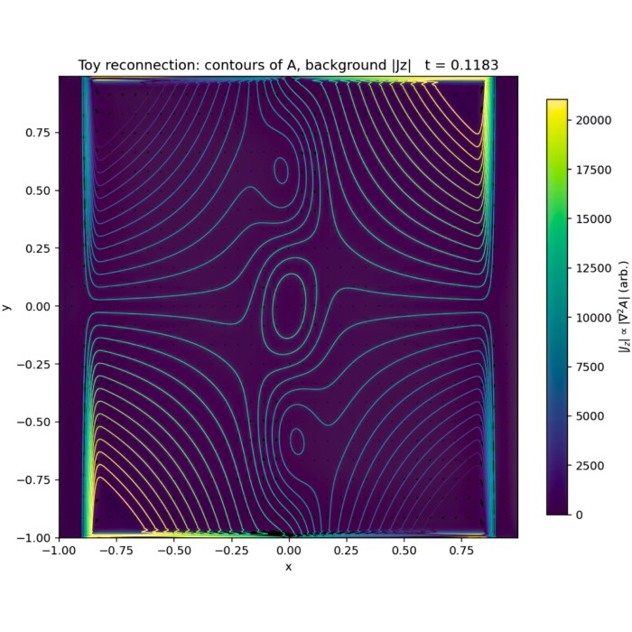
Time evolution of a two-dimensional kinematic reconnection toy model based on X-point collapse. Shown are contours of the magnetic flux function $A(x,y,t)$, representing magnetic field lines, overlaid on the magnitude of the out-of-plane current density proxy $|J_z| \propto |\nabla^2 A|$ (color scale). A prescribed incompressible stagnation-point flow advects the magnetic field toward the X-point, thinning the current layer and enhancing gradients until resistive diffusion becomes effective and magnetic topology changes. The flow is externally imposed and not evolved self-consistently; the model therefore illustrates the geometric and topological aspects of reconnection rather than full magnetohydrodynamic feedback. Initial, intermediate, and final frames are shown, corresponding to progressive X-point collapse and reconnection.
Interpretation and relation to our first model
Despite these differences, both models describe the same underlying physical idea: Magnetic flux is advected by a flow, gradients intensify, and resistive diffusion enables a change in field-line connectivity. What differs is the narrative emphasis.
The Harris-sheet model used in the previous model is optimized for didactic clarity. It reproduces the standard inflow–diffusion–outflow structure in a localized region and aligns closely with textbook diagrams of Sweet–Parker–type reconnection.
The X-point collapse model presented here instead highlights how reconnection can arise from the deformation of an existing magnetic null under large-scale driving. It is closer in spirit to classical analytical treatments of X-point collapse and demonstrates how reconnection can be triggered even without an initially extended current sheet.
Taken together, the two models are best viewed as complementary. They do not represent different reconnection mechanisms, but rather different idealized geometries and driving conditions within the same reduced physical framework. Showing both side by side helps clarify which features of reconnection are robust consequences of resistive induction, and which depend on the specific geometry and assumptions imposed on the system.
Update and code availability: This post and its accompanying Python code were originally drafted in 2020 and archived during the migration of this website to Jekyll and Markdown. In January 2026, I substantially revised and extended the code. The updated and cleaned-up implementation is now available in this new GitHub repositoryꜛ. Please feel free to experiment with it and to share any feedback or suggestions for further improvements.
References and further reading
- Wolfgang Baumjohann and Rudolf A. Treumann, Basic Space Plasma Physics, 1997, Imperial College Press, ISBN: 1-86094-079-X
- J. A. Bittencourt, Fundamentals of Plasma Physics, 2004, Springer, ISBN: 978-0-387-20975-3
- Wikipedia article on Magnetic Reconnectionꜛ


comments