Kelvin–Helmholtz instability in 2D incompressible shear flows

In space physics, a surprisingly large class of phenomena can be understood using the classical equations of hydrodynamics. The main conceptual extension required to describe plasmas is the coupling of the fluid equations to electromagnetic fields via Maxwell’s equations. In a deliberately simplified view, magnetohydrodynamics can be regarded as hydrodynamics with electric and magnetic fields switched on.

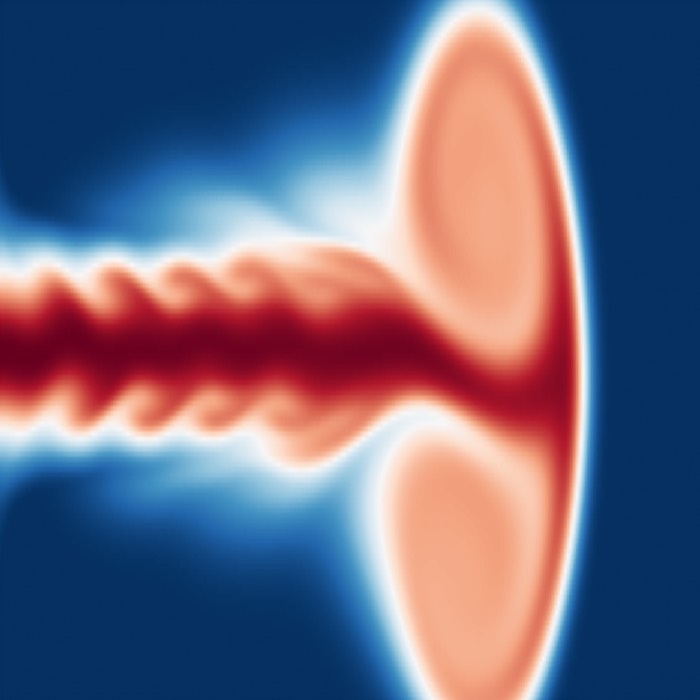
Example of a spatially developping 2D Kelvin-Helmholtz instability. Small perturbations, imposed at the inlet on the tangential velocity, evolve in the computational box. The simulation is run at a low Reynolds number. Source: Wikimedia Commonsꜛ (license: public domain).

When we discussed, for instance, plasma instabilities in this context, we encountered a phenomenon known as the Kelvin–Helmholtz instability. In hydrodynamics, this instability arises at the interface between two fluid layers that slide past each other with different velocities. Small perturbations at the interface can grow over time, leading to the formation of characteristic rolling vortices. In magnetized plasmas, it appears in many astrophysical and heliospheric settings, including velocity shears at planetary magnetopauses, along current sheets, or at the boundaries of astrophysical jets.

In this post, I’d like to introduce this instability from its original viewpoint of classical fluid dynamics. Stripping away magnetic fields and plasma-specific effects we will focus on the essential mechanism of shear-driven instability and vortex formation, accompanied by a simple numerical example implemented in Python.

Physical description

The Kelvin–Helmholtz instability arises when two fluid layers move past each other with different velocities. This usually occurs at the interface between the layers of a stratified fluid or within a continuous shear layer, where the velocity changes smoothly over a finite thickness. If a sufficiently strong velocity shear exists across an interface or within a finite shear layer, small perturbations at that interface can extract kinetic energy from the mean flow and grow exponentially in time.

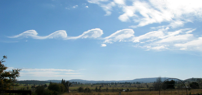
A Kelvin-Helmholtz instability rendered visible by clouds, known as fluctus, over Mount Duval in Australia. Source: Wikimedia Commonsꜛ (license: CC BY-SA 3.0).

In the simplest idealization, two inviscid fluids of equal density slide past each other with a discontinuous velocity jump. In that limit, the interface is unstable for arbitrarily small perturbations at all wavelengths. Realistic flows, however, always possess a finite shear-layer thickness and nonzero viscosity. These effects regularize the instability and introduce preferred length and time scales.

A Kelvin-Helmholtz instability on Saturn, formed at the interaction of two bands of the planet’s atmosphere. Source: Wikimedia Commonsꜛ (license: public domain).

Physically, the instability can be understood as follows. A small transverse displacement of the interface locally tilts the velocity profile. Pressure adjusts to maintain continuity, but this adjustment reinforces the original perturbation rather than restoring it. As the perturbation grows, vorticity concentrates and rolls up into coherent vortices. At later stages, these vortices may interact, merge, or break down into more complex flow structures.

Animation of the KH instability, using a second order 2D finite volume scheme. Source: Wikimedia Commonsꜛ (license: CC BY-SA 4.0).

In many natural systems, including atmospheric flows, ocean currents, and space and astrophysical plasmas, Kelvin–Helmholtz instability acts as a gateway from ordered shear flows to turbulence and enhanced mixing.

Mathematical description

To prepare for the numerical example, we briefly outline the mathematical formulation of the Kelvin–Helmholtz instability in a two-dimensional incompressible shear flow. We start from the incompressible Navier–Stokes equations for a constant-density fluid,

\[\begin{aligned} \partial_t \mathbf{u} + \mathbf{u} \cdot \nabla \mathbf{u} &= -\frac{1}{\rho} \nabla p + \nu \nabla^2 \mathbf{u} + \mathbf{F}(x,y,t), \\ \nabla \cdot \mathbf{u} &= 0, \end{aligned}\]

where $\rho$ is constant, $\nu$ is the kinematic viscosity, and $\mathbf{F}$ is an external body force per unit mass.

In such settings, it is often convenient to work with the vorticity field $\omega = \partial_x v - \partial_y u$ rather than the velocity field $\mathbf{u} = (u,v)$. Taking the curl of the momentum equation yields a scalar evolution equation for $\omega(x,y,t)$,

\[\partial_t \omega + \mathbf{u} \cdot \nabla \omega = \nu \nabla^2 \omega + F(x,y,t),\]

where $F(x,y,t) = (\nabla \times \mathbf{F})_z$ is the out-of-plane curl of the forcing. In the numerical example below we directly prescribe $F$ as a localized vorticity source term.

The velocity field $\mathbf{u} = (u,v)$ is obtained from a scalar streamfunction $\psi(x,y,t)$ via

\[u = \partial_y \psi, \qquad v = -\partial_x \psi,\]

which automatically enforces incompressibility, $\nabla \cdot \mathbf{u} = 0$. The streamfunction itself is related to vorticity through the Poisson equation

\[\nabla^2 \psi = -\omega.\]

This formulation removes the pressure from the equations and reduces the problem to a single scalar evolution equation coupled to an elliptic constraint.

Base flow and perturbations

In our numerical example, we consider a base flow consisting of a planar shear layer with a hyperbolic tangent velocity profile:

\[u_0(y) = U_{\text{mean}} + U_0 \tanh\!\left(\frac{y - y_0}{\delta}\right),\]

$u_0(y)$ represents two parallel streams separated by a shear layer of thickness $\delta$. The parameter $U_{\text{mean}}$ introduces a uniform downstream advection, while $U_0$ controls the shear strength. The associated base-state vorticity is

\[\omega_0(y) = -\frac{\mathrm{d}u_0}{\mathrm{d}y}.\]

Kelvin–Helmholtz instability is triggered by superimposing small transverse perturbations on this base flow. In the numerical setup, these perturbations are localized in the streamwise direction near $x \approx 0$, mimicking a weakly disturbed inlet region rather than a globally perturbed interface.

Numerical discretization

For our numerical simulation, we need to decide for a numerical method to solve the vorticity equation. In this example, we employ a pseudospectral method with Fourier discretization in both spatial directions. The computational domain is a rectangular box of size $L_x \times L_y$, discretized using $N_x \times N_y$ grid points with periodic boundary conditions in both directions. For such a periodic domain, the Laplacian and first derivatives become algebraic operations in Fourier space, allowing highly accurate evaluation of gradients. We came already accross spectral methods in our post on “A spectral (FFT) Poisson solver for 1D electrostatic PIC”.

Nonlinear advection terms are computed in physical space, where products of fields are evaluated pointwise. To prevent aliasing errors inherent to pseudospectral methods, the nonlinear term is dealiased using the standard two-thirds rule. This step is essential for numerical stability once vortices sharpen and small scales emerge.

Time integration is then performed using an explicit second-order Runge–Kutta scheme. The time step is chosen adaptively based on a Courant–Friedrichs–Lewy condition derived from the instantaneous velocity field,

\[\Delta t \le C \min\!\left(\frac{\Delta x}{|u|_{\max}}, \frac{\Delta y}{|v|_{\max}}\right),\]

with a safety factor $C < 1$. This prevents numerical instabilities due to excessive advection within a single time step. As a consequence, the time step decreases as vortices form and flow speeds increase locally, i.e., there is no fixed time step throughout the simulation.

Boundary conditions and their implications

We choose the computational domain to be periodic in both spatial directions. This choice is dictated by the spectral discretization, which requires periodicity to retain its efficiency and simplicity.

As a consequence, the system will possess no physical inlet or outlet boundaries. Structures advected out of the domain re-enter on the opposite side. The localized perturbations near $x \approx 0$ therefore act as a persistent source region rather than a true boundary condition.

This has important interpretational consequences. Although the mean flow introduces a preferred downstream direction and the perturbations are spatially localized, the evolution is only quasi spatially developing. Vortices may appear anywhere in the domain, including near the right edge, without indicating a physical interaction with a boundary.

Numerical example with Python

The numerical example below implements the above-described setup in Python. It simulates the development of Kelvin–Helmholtz instability in a two-dimensional incompressible shear flow using a pseudospectral method with periodic boundary conditions.

In the following, we will walk through the code step by step, explaining the key components and their roles in the simulation. The complete code is provided in the GitHub repository mentioned at the end of this post.

We begin by importing the necessary libraries and setting up some global plotting parameters for better aesthetics:

import os
import numpy as np
import matplotlib.pyplot as plt
import imageio.v2 as imageio

# remove spines right and top for better aesthetics:
plt.rcParams['axes.spines.right'] = False
plt.rcParams['axes.spines.top'] = False
plt.rcParams['axes.spines.left'] = False
plt.rcParams['axes.spines.bottom'] = False
plt.rcParams.update({'font.size': 12})

As first helper function, we define a routine to compute the FFT wavenumbers for a given grid size and domain length:

def make_wavenumbers(n: int, L: float) -> np.ndarray:
    """
    FFT wavenumbers in rad per length.
    """
    return 2.0 * np.pi * np.fft.fftfreq(n, d=L / n)

Next, we implement functions to compute spectral derivatives in the x and y directions using the Fourier transform:

def spectral_derivative_x(f_hat: np.ndarray, kx: np.ndarray) -> np.ndarray:
    """
    Compute d/dx of a field given its Fourier transform along x and y (2D FFT).
    """
    return np.fft.ifft2(1j * kx[:, None] * f_hat).real


def spectral_derivative_y(f_hat: np.ndarray, ky: np.ndarray) -> np.ndarray:
    """
    Compute d/dy of a field given its Fourier transform along x and y (2D FFT).
    """
    return np.fft.ifft2(1j * ky[None, :] * f_hat).real

Then, we define a function to compute the spectral Laplacian of a field in Fourier space:

def laplacian_hat(f_hat: np.ndarray, kx: np.ndarray, ky: np.ndarray) -> np.ndarray:
    """
    Spectral Laplacian: -(kx^2 + ky^2) * f_hat
    """
    k2 = (kx[:, None] ** 2) + (ky[None, :] ** 2)
    return -(k2) * f_hat

We also need a function to solve the Poisson equation for the streamfunction given the vorticity field:

def poisson_solve_streamfunction(omega: np.ndarray, kx: np.ndarray, ky: np.ndarray) -> np.ndarray:
    """
    Solve ∇^2 ψ = -ω in Fourier space on a periodic domain:
    ψ_hat = ω_hat / (kx^2 + ky^2), with zero mode set to 0.
    """
    omega_hat = np.fft.fft2(omega)
    k2 = (kx[:, None] ** 2) + (ky[None, :] ** 2)
    psi_hat = np.zeros_like(omega_hat, dtype=np.complex128)

    mask = k2 > 0.0
    psi_hat[mask] = omega_hat[mask] / k2[mask]
    psi_hat[~mask] = 0.0

    psi = np.fft.ifft2(psi_hat).real
    return psi

and a function to compute the velocity field from the streamfunction:

def compute_velocity_from_streamfunction(psi: np.ndarray, kx: np.ndarray, ky: np.ndarray) -> tuple[np.ndarray, np.ndarray]:
    """
    u =  dψ/dy, v = -dψ/dx
    """
    psi_hat = np.fft.fft2(psi)
    u = spectral_derivative_y(psi_hat, ky)
    v = -spectral_derivative_x(psi_hat, kx)
    return u, v

To implement dealiasing for the nonlinear term, we create a mask that retains only the lower two-thirds of the wavenumbers:

def make_dealias_mask(Nx: int, Ny: int) -> np.ndarray:
    """
    2/3-rule dealiasing mask for 2D FFT grids.
    Keeps modes |k| <= N/3 in each direction.
    """
    kx_idx = np.fft.fftfreq(Nx) * Nx
    ky_idx = np.fft.fftfreq(Ny) * Ny
    kx_max = Nx // 3
    ky_max = Ny // 3
    mask = (np.abs(kx_idx)[:, None] <= kx_max) & (np.abs(ky_idx)[None, :] <= ky_max)
    return mask.astype(float)

For our RK2 time-stepping, we need to define the right-hand side of the vorticity equation:

def rhs_vorticity(omega: np.ndarray, nu: float, kx: np.ndarray, ky: np.ndarray, forcing: np.ndarray,
                  dealias_mask: np.ndarray | None = None) -> np.ndarray:
    """
    Right-hand side: -u·∇ω + ν∇^2 ω + forcing
    """
    psi = poisson_solve_streamfunction(omega, kx, ky)
    u, v = compute_velocity_from_streamfunction(psi, kx, ky)

    omega_hat = np.fft.fft2(omega)
    domega_dx = spectral_derivative_x(omega_hat, kx)
    domega_dy = spectral_derivative_y(omega_hat, ky)

    adv = u * domega_dx + v * domega_dy

    # dealias advection term (important for stability of pseudospectral nonlinear products):
    if dealias_mask is not None:
        adv_hat = np.fft.fft2(adv)
        adv_hat *= dealias_mask
        adv = np.fft.ifft2(adv_hat).real

    lap_omega = np.fft.ifft2(laplacian_hat(omega_hat, kx, ky)).real

    return -adv + nu * lap_omega + forcing

The next couple of functions handle figure rendering and conversion to RGB arrays for saving frames:

def fig_to_rgb_array(fig) -> np.ndarray:
    """
    Convert a Matplotlib figure to an RGB uint8 image array of shape (H, W, 3).
    Works across Matplotlib backends/versions using buffer_rgba().
    """
    fig.canvas.draw()
    w, h = fig.canvas.get_width_height()

    # RGBA buffer, length = w*h*4
    buf = np.asarray(fig.canvas.buffer_rgba(), dtype=np.uint8).reshape((h, w, 4))

    # Drop alpha channel
    rgb = buf[:, :, :3].copy()
    return rgb

def render_frame(x, y, omega, t, vmin=None, vmax=None):
    fig, ax = plt.subplots(figsize=(8.4, 4.6), dpi=140)
    extent = [x.min(), x.max(), y.min(), y.max()]

    im = ax.imshow(omega.T, origin="lower", extent=extent, aspect="auto",
        vmin=vmin, vmax=vmax,cmap="RdBu_r",)
    ax.set_xlabel("x")
    ax.set_ylabel("y")
    ax.set_title(f"2D Kelvin-Helmholtz vorticity  t = {t:.3f}")

    cbar = fig.colorbar(im, ax=ax)
    cbar.set_label("vorticity ω")

    fig.tight_layout()
    rgb = fig_to_rgb_array(fig)
    plt.close(fig)
    return rgb

Having now everything in place, we can set up the main simulation parameters. We first define the computational domain and grid:

Nx = 512        # number of grid points in x
Ny = 256        # number of grid points in y
Lx = 300.0      # domain length in x
Ly = 70.0       # domain length in y

x = np.linspace(0.0, Lx, Nx, endpoint=False)
y = np.linspace(0.0, Ly, Ny, endpoint=False)
X, Y = np.meshgrid(x, y, indexing="ij")

kx = make_wavenumbers(Nx, Lx)
ky = make_wavenumbers(Ny, Ly)

dx = Lx / Nx    # grid spacing in x
dy = Ly / Ny    # grid spacing in y

Then, we set the basic physical parameters such as the shear velocity, viscosity, and time-stepping parameters. We also ste the CFL control parameters for the adaptive time-stepping:

# physical parameters:
U0 = 2.5           # shear velocity scale, start with 1.0, then increase for higher Re
Umean = 2.0        # net advection to +x
delta = 1.5        # shear layer thickness scale
nu = 0.012         # viscosity (choose larger for lower Reynolds number)

# time stepping:
dt = 0.05
nsteps = 2200

# CFL control (stability):
cfl = 0.30
dt_max = 0.03
dt_min = 1e-4

We set the base shear profile and initialize the vorticity field with a small localized perturbation near the inlet:

# base shear profile u0(y):
y0 = 0.5 * Ly
u0 = Umean + U0 * np.tanh((y - y0) / delta)
du0_dy = (U0 / delta) * (1.0 / np.cosh((y - y0) / delta) ** 2)
omega0_y = -du0_dy  # ω = ∂v/∂x - ∂u/∂y, base has v=0, u=u(y)

omega = np.repeat(omega0_y[None, :], Nx, axis=0)

We also add a small initial perturbation to the vorticity field to seed the instability:

# spatially localized initial perturbation near the "inlet" x ~ 0:
eps0 = 0.25
x_loc = 18.0
sigma_x = 14.0
ky_mode = 2.0 * np.pi / Ly * 3.0

inlet_envelope = np.exp(-((X - x_loc) ** 2) / (2.0 * sigma_x ** 2))
omega += eps0 * inlet_envelope * np.sin(ky_mode * Y)

In the main simulation loop, we optionally include a time-dependent forcing term that mimics continuous perturbations at the inlet:

# optional time-dependent inlet forcing F(x,y,t)
forcing_on = True
epsF = 0.10
forcing_sigma_x = 10.0
forcing_x0 = 8.0
forcing_omega_t = 0.35
forcing_ky_mode = 2.0 * np.pi / Ly * 5.0

forcing_x_env = np.exp(-((X - forcing_x0) ** 2) / (2.0 * forcing_sigma_x ** 2))

Apart from the the physical parameters, we also need to define the output control parameters for saving simulation frames before we start the actual time integration:

# output control:
frame_every = 10
frames_dir = "khi_periodic_BC_frames"
gif_path = "kelvin_helmholtz_2d.gif"
gif_path = "kelvin_helmholtz_2d.gif"
os.makedirs(frames_dir, exist_ok=True)

# determine a stable plotting range from the initial field
q = np.quantile(np.abs(omega), 0.995)
vmin, vmax = -q, q

In our main time integration loop, which is the next block in our code, will perform the RK2 time-stepping, i.e., temporal integration of the vorticity equation, incorporating the adaptive time step based on the CFL condition. We also save frames at regular intervals for later visualization:

# time integration (RK2)

# create storage for output frames:
frame_paths = []
frame_idx = 0

# initialize a GIF writer:
writer = imageio.get_writer(gif_path, mode="I", duration=0.05, loop=0)

# dealiasing mask for nonlinear term:
dealias_mask = make_dealias_mask(Nx, Ny)

# set initial time:
t = 0.0

try:
    for n in range(nsteps + 1):

        # compute velocity for CFL-based adaptive dt:
        psi = poisson_solve_streamfunction(omega, kx, ky)
        u, v = compute_velocity_from_streamfunction(psi, kx, ky)
        umax = np.max(np.abs(u))
        vmax_loc = np.max(np.abs(v))
        speed_eps = 1e-12

        dt_cfl = cfl * min(dx / (umax + speed_eps), dy / (vmax_loc + speed_eps))
        dt = float(np.clip(dt_cfl, dt_min, dt_max))

        if forcing_on:
            forcing = epsF * forcing_x_env * np.sin(forcing_ky_mode * Y) * np.sin(forcing_omega_t * t)
        else:
            forcing = np.zeros_like(omega)

        # save frame every frame_every steps:
        if (n % frame_every) == 0:
            rgb = render_frame(x, y, omega, t, vmin=vmin, vmax=vmax)

            outpath = os.path.join(frames_dir, f"frame_{frame_idx:05d}.png")
            imageio.imwrite(outpath, rgb)     # PNG from the exact same pixels
            writer.append_data(rgb)           # GIF frame from RAM

            frame_idx += 1
            print(f"Saved {outpath}")

        # RK2 step:
        k1 = rhs_vorticity(omega, nu, kx, ky, forcing, dealias_mask=dealias_mask)
        omega_tmp = omega + dt * k1

        if forcing_on:
            forcing2 = epsF * forcing_x_env * np.sin(forcing_ky_mode * Y) * np.sin(forcing_omega_t * (t + dt))
        else:
            forcing2 = np.zeros_like(omega)

        k2 = rhs_vorticity(omega_tmp, nu, kx, ky, forcing2, dealias_mask=dealias_mask)
        omega = omega + 0.5 * dt * (k1 + k2)

        if not np.isfinite(omega).all():
            print(f"Non-finite omega encountered at step {n}, t={t:.3f}. Aborting.")
            break

        t += dt

finally:
    writer.close()

The loop above runs as follows: It will first compute the maximum velocity in the domain to determine a stable time step based on the CFL condition. If forcing is enabled, it computes the forcing term at the current time. Every frame_every steps, it renders and saves a frame of the vorticity field. The RK2 time-stepping is then performed, updating the vorticity field for the next time step. If any non-finite values are encountered in the vorticity field, the simulation aborts.

Discussion of the numerical example

The reuslting GIF animation below compiles all saved frames and illustrates the full temporal evolution of the Kelvin–Helmholtz instability in the two-dimensional incompressible shear flow:

Compiled GIF animation of the 2D Kelvin-Helmholtz instability simulation showing the vorticity field evolution over time.

To discuss the observed dynamics, we will walk through the key stages of the instability by presenting selected snapshots from the simulation. Each vorticity snapshots illustrates the dynamical evolution of the two-dimensional Kelvin–Helmholtz unstable shear layer governed by the vorticity equation

\[\partial_t \omega + \mathbf{u} \cdot \nabla \omega = \nu \nabla^2 \omega + F(x,y,t),\]

with the velocity field $\mathbf{u} = (u,v)$ obtained from the streamfunction $\psi$ via $u = \partial_y \psi$ and $v = -\partial_x \psi$.

Initial state and linear regime

At $t = 0$, the flow is dominated by the base-state vorticity

\[\omega_0(y) = -\frac{\mathrm{d}u_0}{\mathrm{d}y},\]

which appears as a narrow, horizontally aligned vorticity sheet centered around $y \approx y_0$. The imposed perturbation is weak and spatially localized near $x \approx 0$, producing only small-amplitude vorticity fluctuations superimposed on the base profile. At this stage, the dynamics are well described by the linearized vorticity equation around $\omega_0(y)$, and advection by the mean flow $U_{\text{mean}}$ transports perturbations downstream without significant deformation.

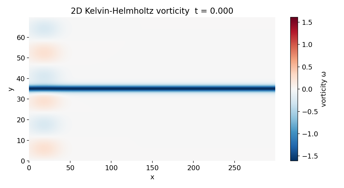
Initial vorticity field at $t = 0$. The flow is dominated by the base-state vorticity $\omega_0(y) = -\mathrm{d}u_0/\mathrm{d}y$, appearing as a narrow, horizontally aligned vorticity sheet centered at $y \approx y_0$. Small-amplitude perturbations are confined to a localized region near $x \approx 0$ and remain in the linear regime.

Onset of Kelvin–Helmholtz instability

By $t \approx 15$, the initially small perturbations have grown sufficiently for the shear layer to exhibit visible undulations. This marks the transition from the linear to the weakly nonlinear Kelvin–Helmholtz regime. The instability extracts kinetic energy from the velocity shear $\partial_y u_0$, converting it into growing transverse displacements of the vorticity sheet. The growth is most pronounced where perturbations were initially seeded, but advection by $U_{\text{mean}}$ spreads these disturbances along the streamwise direction.

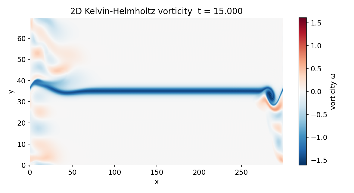
Vorticity field at $t \approx 15$. The initially flat shear layer begins to undulate as Kelvin–Helmholtz modes grow by extracting energy from the velocity shear $\partial_y u_0$. The deformation remains smooth, indicating that the dynamics are transitioning from the linear to the weakly nonlinear regime.

The characteristic feature of this phase is the bending of the vorticity layer into a sinusoidal shape. At this point, nonlinear advection $\mathbf{u} \cdot \nabla \omega$ becomes comparable to viscous diffusion $\nu \nabla^2 \omega$, and mode coupling begins to play an important role.

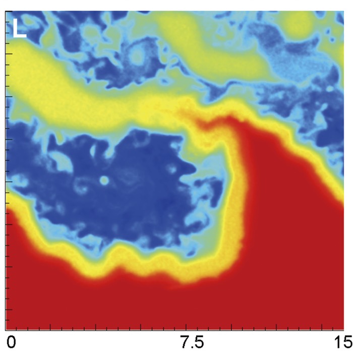
Vortex roll-up and nonlinear saturation

At later times, $t \approx 30$ to $40$, the shear layer undergoes classical Kelvin–Helmholtz roll-up. The vorticity sheet locally concentrates and curls into coherent vortices with alternating sign. This roll-up reflects the nonlinear saturation of the instability. Once vortices form, they modify the local velocity field $\mathbf{u}$, which in turn feeds back on the vorticity through the advection term.

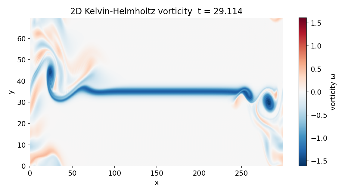
Vorticity field at $t \approx 29$. Nonlinear advection $\mathbf{u}\cdot\nabla\omega$ becomes dominant locally, and the shear layer starts to roll up into distinct vortical structures. Concentration of vorticity marks the formation of the first coherent Kelvin–Helmholtz vortices.

During this phase, the flow develops a hierarchy of spatial scales. Sharp vorticity gradients appear near the vortex cores, while elongated filaments connect neighboring structures. Viscous diffusion acts to smooth the smallest scales, but at the chosen Reynolds number the vortices remain well defined over long times. The adaptive time step enforced through the CFL condition reflects this increasing complexity, decreasing as local velocities and gradients grow.

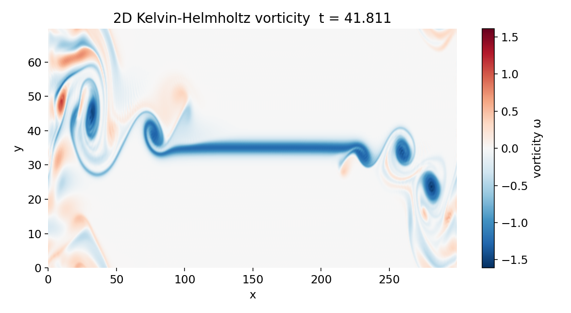
Vorticity field at $t \approx 42$. The instability has saturated into well-defined vortices connected by elongated vorticity filaments. Strong curvature of the original shear layer reflects sustained nonlinear interactions, while viscous diffusion limits the growth of the smallest scales.

Long-time evolution and interaction across the domain

By $t \approx 60$, the flow has entered a fully nonlinear regime characterized by interacting vortices and extended vorticity filaments. Vortices generated near the initial perturbation region have been advected downstream, while new structures continue to emerge from the shear layer. Importantly, coherent vortices are now visible near both the left and right edges of the domain.

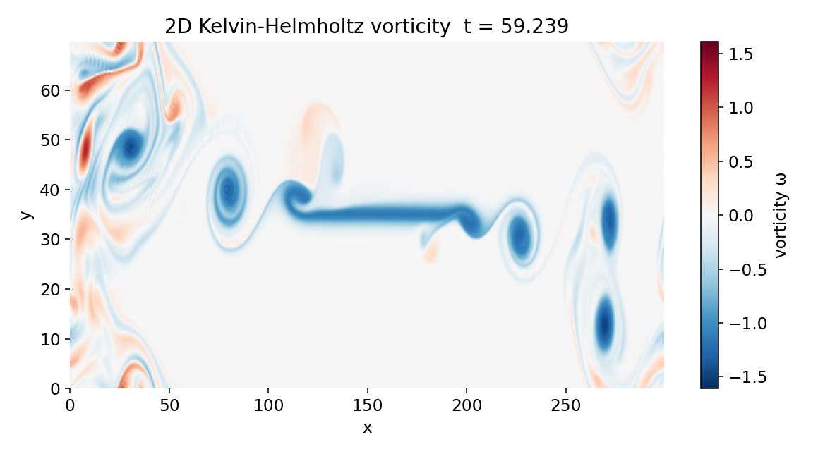
Vorticity field at $t \approx 59$. Multiple vortices coexist and interact across the entire domain. Structures appearing near the domain boundaries reflect periodic boundary conditions, with vortices advected out of the domain re-entering on the opposite side. The flow exhibits fully nonlinear Kelvin–Helmholtz dynamics with sustained vortex interaction.

This behavior is a direct consequence of the periodic boundary conditions in the streamwise direction. Structures advected out of the domain at large $x$ re-enter at small $x$ without loss of coherence. As a result, the localized perturbation near $x \approx 0$ acts as a persistent source of disturbances rather than a true inlet, and the domain supports a repeating pattern of shear-layer destabilization and vortex formation.

Implications of periodic boundary conditions

The periodicity in $x$ and $y$ has two important implications for the interpretation of the results. First, the simulation does not represent a strictly spatially developing Kelvin–Helmholtz instability with a physical inflow and outflow. Instead, it describes a quasi spatially developing shear layer embedded in a repeating domain. This means, that vortices can appear anywhere in the domain, not just downstream of the initial perturbation region. Second, the appearance of vortices near the right boundary does not indicate reflection or boundary interaction, but simply the re-entry of advected structures.

From a numerical perspective, these boundary conditions greatly simplify the solution of the Poisson equation $\nabla^2 \psi = -\omega$ and enable an efficient and spectrally accurate discretization. Physically, they allow the focus to remain on the intrinsic instability and nonlinear vortex dynamics, rather than on boundary-layer effects or outflow treatment.

Summary of the observed dynamics

Overall, the snapshots we have discussed above capture the canonical stages of the Kelvin–Helmholtz instability: Linear growth of perturbations on a shear layer, nonlinear roll-up into vortices, and subsequent vortex interaction and filamentation. The vorticity–streamfunction formulation provides a particularly clear view of these processes, as vorticity directly highlights the regions where shear is concentrated and where instability-driven dynamics are most active.

The simulation thus serves as a controlled numerical experiment that isolates the fundamental hydrodynamic mechanisms underlying Kelvin–Helmholtz instability, while remaining closely connected to the mathematical structure of the governing equations introduced earlier.

Conclusion

Kelvin–Helmholtz instability is one of the clearest examples of how a seemingly simple ingredient, a velocity shear, can destabilize an otherwise ordered flow and generate coherent structure. In the incompressible setting considered here, the mechanism is fully contained in the nonlinear vorticity dynamics

\[\partial_t \omega + \mathbf{u}\cdot\nabla\omega = \nu\nabla^2\omega + F(x,y,t),\]

together with the elliptic coupling between vorticity and velocity through the streamfunction,

\[\begin{aligned} \nabla^2\psi&=-\omega,\\ u&=\partial_y\psi,\\ v&=-\partial_x\psi. \end{aligned}\]

Once a shear layer establishes a strong gradient $\partial_y u_0$, small transverse disturbances can tap into the kinetic energy of the mean flow and grow. In the simulation, this growth first appears as smooth undulations of the vorticity sheet $\omega_0(y)=-\mathrm{d}u_0/\mathrm{d}y$, then transitions into nonlinear roll up where $\mathbf{u}\cdot\nabla\omega$ concentrates vorticity into vortex cores and filaments. At later times, the dynamics are dominated by vortex interaction, advection, and viscous smoothing, with $\nu\nabla^2\omega$ setting the smallest resolved length scale.

The numerical example also makes explicit what is gained and what is sacrificed by the periodic Fourier based discretization. Periodicity yields a particularly clean and efficient solver because derivatives and the Poisson inversion are algebraic in Fourier space. At the same time, the periodic boundary conditions imply that the setup is not a strictly spatially developing inlet outlet problem, even if the perturbations are localized near $x\approx 0$ and the base profile includes a net advection $U_{\text{mean}}$. Structures leaving the domain re-enter on the opposite side, so vortices near the right boundary should be interpreted as advected and wrapped around structures, not as a boundary interaction. For the purpose of isolating the intrinsic Kelvin–Helmholtz dynamics, we accepted this tradeoff in our example.

Finally, returning to the space physics motivation, the main conceptual message is that much of the qualitative phenomenology of shear driven mixing and vortex formation already follows from classical hydrodynamics. In magnetized plasmas, additional physics can suppress, reshape, or channel Kelvin–Helmholtz growth, but the basic shear extraction mechanism remains the reference point. I think, understanding the fluid case in a mathematically transparent formulation provides a solid baseline for interpreting Kelvin–Helmholtz type signatures at magnetopauses, current sheets, and other shear interfaces once electromagnetic forces are added.

I am currently preparing Here is a follow-up post takes our example provided here as a starting point and solves the problem by applying a finite-volume method on a staggered grid with physical inflow and outflow boundary conditions. This will allow us to directly simulate a spatially developing Kelvin–Helmholtz instability and compare the results to the periodic case discussed here. Stay tuned!

Update and code availability: This post and its accompanying Python code were originally drafted in 2021 and archived during the migration of this website to Jekyll and Markdown. In January 2026, I substantially revised and extended the code. The updated and cleaned-up implementation is now available in this new GitHub repositoryꜛ. Please feel free to experiment with it and to share any feedback or suggestions for further improvements.

References and further reading

• Walter Greiner, Horst Stock, Hydrodynamik - Ein Lehr- und Übungsbuch; mit Beispielen und Aufgaben mit ausführlichen Lösungen, 1991, Harri Deutsch Verlag, ISBN: 9783817112043
• Heinz Schade and Ewald Kunz, Strömungslehre, 2007, de Gruyter, ISBN: 978-3-11-018972-8
• Sirovich Antman, J. E. Marsden, Hale P Holmes, J. Keller, J. Keener, B. J. Mielke, A. Matkowsky, C. S. Sreenivasan, and K. R. S. Perkin, Prandtl’s Essential of Fluid Mechanics, 2004, Vol. 158, Springer, ISBN: 0-387-40437-6
• O. G. Drazin, Introduction to hydrodynamic stability, 2002, Cambridge University Press, ISBN: 0521 80427 2
• Rutherford Aris, Vectors, tensors and the basic equations of fluid mechanics, 1962, Dover Publications Inc., ISBN: 0-486-66110-5
• Jianping Zhu, Computational Simulations and Applications, 2011, Intechweb.org, ISBN: 978-953-307-430-6
• Pieter Wesseling, Principles of computational fluid dynamics, 2001, Springer-Verlag, ISBN: 3-540-67853-0
• Franz Durst, Grundlagen der Strömungslehre, 2006, Springer-Verlag, ISBN: 978-3-540-31323-6
• Wilhelm Kley, Numerische Hydrodynamik, 2004, Universitaet Tuebingen (Lecture Notes)
• Burg, K., Haf, H., Wille, F., & Meister, A. Partielle Differentialgleichungen und funktionalanalytische Grundlagen, 2010, 5th ed., Vieweg + Teubner, ISBN: 978-3-8348-1294-0
• Lord Kelvin (William Thomson), Hydrokinetic solutions and observations, 1871, Philosophical Magazine. 42: 362–377
• Hermann von Helmholtz, Über discontinuierliche Flüssigkeits-Bewegungen [On the discontinuous movements of fluids]”, 1868, Monatsberichte der Königlichen Preussische Akademie der Wissenschaften zu Berlin. 23: 215–228
• Wikipedia article on Kelvin–Helmholtz instabilityꜛ