Turbulence, Richardson cascade, and spectral scaling in incompressible flows

Turbulence is a generic dynamical regime of fluids, independent of whether the medium is liquid, gas, or plasma. In this regime, flow fields become highly complex and appear chaotic. Turbulence is a universal feature of geophysical fluids and largely controls their transport properties, including mixing, momentum transport, and the redistribution of energy across length scales. Despite its ubiquity, turbulence remains one of the central unresolved problems of classical physics, because the governing equations are known, but a closed, predictive theory for the multiscale statistics of turbulent flows is not. A widely used phenomenological picture is the Richardson cascade, which views turbulence as an interacting population of vortices, with energy injected on large scales, transferred by nonlinear interactions across an inertial range, and finally dissipated on sufficiently small scales. In this post, we review the basic concepts of turbulence theory, including the Richardson cascade and Kolmogorov’s phenomenological scaling approach. We also discuss practical aspects of spectral analysis in numerical simulations of forced turbulence.

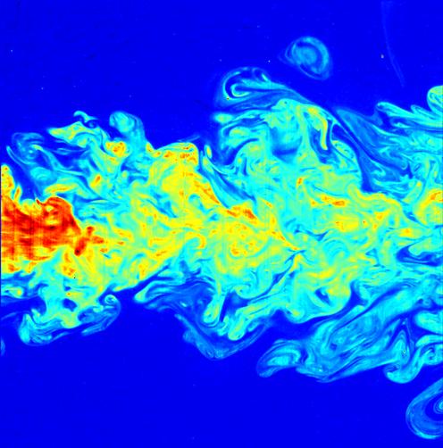
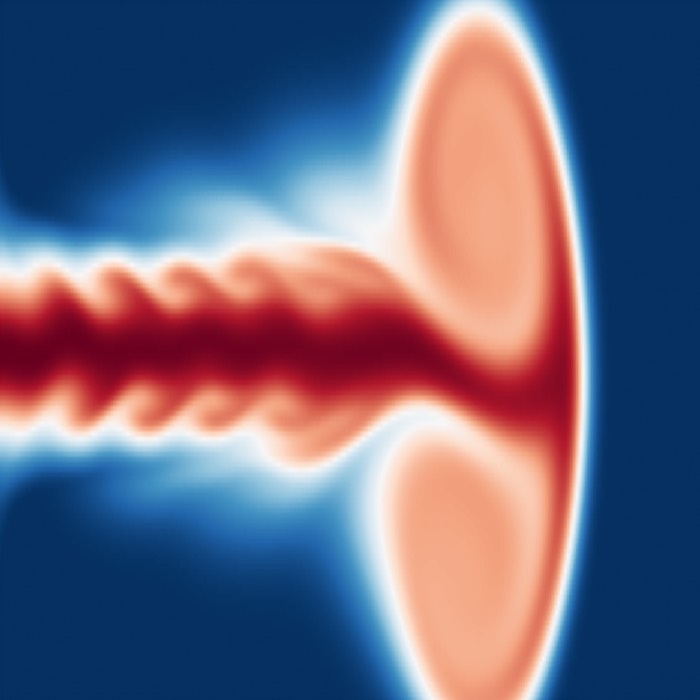
Flow visualization of a turbulent jet, made by laser-induced fluorescence. The jet exhibits a wide range of length scales, an important characteristic of turbulent flows. Source: Wikimedia Commonsꜛ (license: CC BY 3.0).

What is turbulence?

Turbulence is not a separate set of equations, but a regime that emerges from the nonlinear dynamics of the standard fluid equations when inertial effects dominate over viscous dissipation. In the simplest setting considered here, the fluid is incompressible and of constant density. Incompressibility implies

\[\nabla \cdot \mathbf{v} = 0,\]

and constant density implies $\rho = \text{const.}$. Here, $\mathbf{v}(\mathbf{x},t)$ is the fluid velocity field, and $\rho$ is the mass density. The dynamics are governed by the incompressible Navier Stokes equation. Neglecting external body forces and writing the kinematic viscosity as $\nu = \eta / \rho$ yields

\[\begin{align*} \rho \left( \partial_t \mathbf{v} + (\mathbf{v} \cdot \nabla)\mathbf{v} \right) &= -\nabla p + \eta \Delta \mathbf{v} \\ \Leftrightarrow \quad \partial_t \mathbf{v} + (\mathbf{v} \cdot \nabla)\mathbf{v} &= -\frac{1}{\rho} \nabla p + \nu \Delta \mathbf{v}. \end{align*}\]

Here, $\eta$ is the dynamic viscosity, $p(\mathbf{x},t)$ is the fluid pressure, and $\Delta$ is the Laplacian operator. The left hand side contains the inertial terms, while the right hand side contains the pressure gradient force and the viscous diffusion term.

The central source of complexity is the nonlinear advective term $(\mathbf{v} \cdot \nabla)\mathbf{v}$, which couples modes across scales. A standard way to quantify whether nonlinear advection dominates viscous diffusion is the Reynolds number, obtained by comparing the characteristic magnitude of the nonlinear term to the viscous term. With a typical flow speed $v$ and length scale $L$,

\[Re = \frac{\left|(\mathbf{v} \cdot \nabla)\mathbf{v}\right|}{\left|\nu \Delta \mathbf{v}\right|} \sim \frac{v^2/L}{\nu v/L^2} = \frac{L\,v}{\nu}.\]

Here $v$ is a typical flow speed, $L$ is a typical macroscopic length scale such as an obstacle size or integral eddy size, and $\nu$ is the kinematic viscosity. For sufficiently large Reynolds numbers, a wide range of scales becomes dynamically active. A common rule of thumb is that flows become clearly turbulent at $Re \gtrsim 10^3$, though this threshold depends on geometry and forcing.

Numerical simulation of the Navier Stokes equation can reproduce turbulent dynamics, but reproduction is not explanation. The practical approach in turbulence theory is therefore statistical and phenomenological. A key conceptual step is to treat turbulence as a multiscale process in which energy is redistributed across a hierarchy of eddy sizes. This is the content of the Richardson cascade.

The Richardson cascade

The Richardson cascade provides the baseline phenomenological description of fully developed turbulence. Richardson proposed that turbulence can be organized into scale ranges. In this picture, large eddies break down into smaller eddies, which in turn break down further, until viscosity becomes important and dissipates kinetic energy into heat.

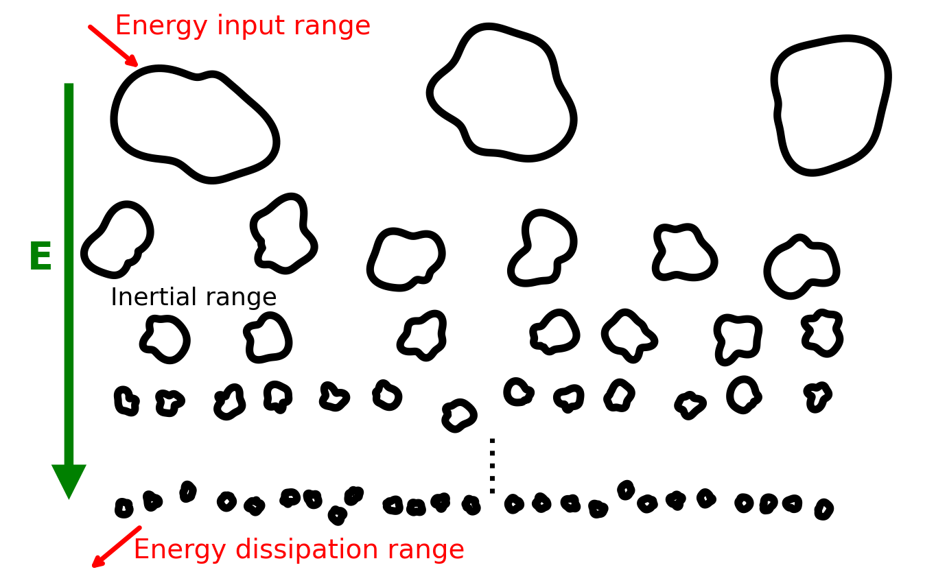
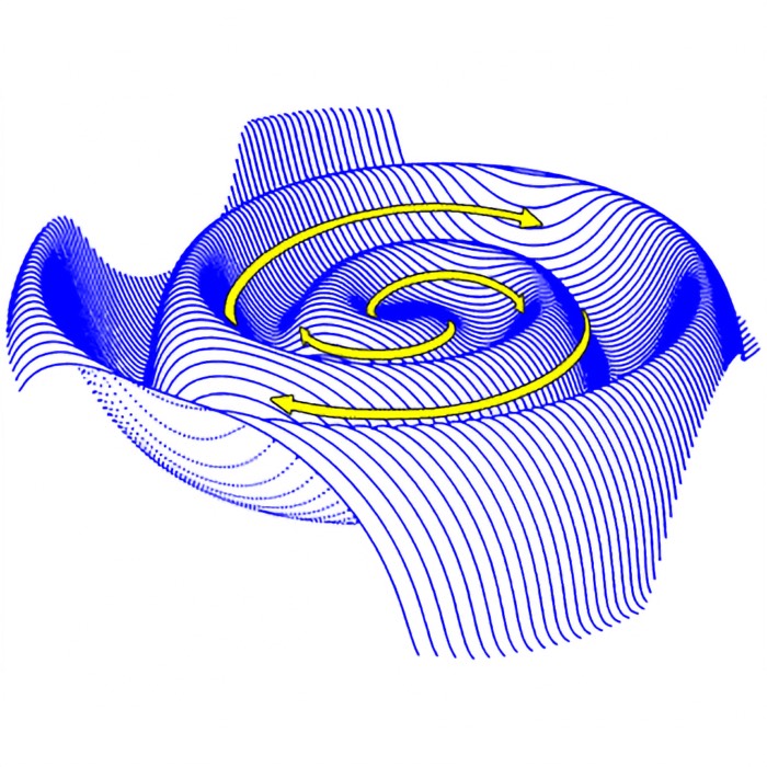
Schematic illustration of the Richardson energy cascade in fully developed turbulence. Energy is injected at large spatial scales in the energy input range, producing large coherent eddies. Through nonlinear advection, these eddies break down into progressively smaller structures across the inertial range, transferring kinetic energy conservatively from large to small scales without dissipation. At sufficiently small scales, corresponding to the energy dissipation range, viscous effects dominate and kinetic energy is irreversibly converted into heat. The vertical arrow indicates the direction of decreasing length scale and energy transfer across scales. The figure is adapted from Lewis Fry Richardson’s original descriptions in his 1922 book Weather Prediction by Numerical Processꜛ (Cambridge University Press. p. 66. ISBN 978-0-511-61829-1). Here, we generated it using a Python script, which you can find in the Github repository mentioned at the end of this post.

A standard separation of scales distinguishes three ranges.

• Production range, also called the integral scale range or energy input range. Energy is injected on the largest dynamically active scales, of order $L$, through boundaries, obstacles, mean shear, or explicit forcing. In a controlled numerical setup, this corresponds to specifying forcing at a prescribed wavenumber band.

• Inertial range. Nonlinear interactions transfer energy across scales without significant direct dissipation. The core assumption is that in this range the energy transfer is conservative in the sense that energy is passed to neighboring scales faster than it can be removed by viscosity. The dynamics in this range are governed primarily by the nonlinear term

  \[\partial_t \mathbf{v} + (\mathbf{v} \cdot \nabla)\mathbf{v}.\]
• Dissipation range. At sufficiently small scales, viscosity becomes dominant and converts kinetic energy into heat. In the Navier Stokes equation, this corresponds to the term $\nu \Delta \mathbf{v}$ becoming comparable to, and then larger than, the nonlinear term.

The Richardson cascade is a qualitative picture, but it motivates quantitative scaling arguments. Kolmogorov’s approach is precisely such a scaling theory for the inertial and dissipation ranges.

Kolmogorov’s phenomenological approach

Kolmogorov’s theory starts from the Richardson cascade and adds a universality hypothesis. The hypothesis states that, sufficiently deep into the cascade, the detailed anisotropic imprint of large scale forcing is progressively lost. If the separation between the large injection scale $L$ and the small dissipation scale is large, meaning $\eta/L$ is small, or equivalently the Reynolds number is large, then small scale turbulence becomes approximately homogeneous and isotropic. Under these conditions, the small scale statistics become universal and are determined only by the scale itself and a small number of parameters.

A central parameter is the mean energy dissipation rate per unit mass, denoted $\epsilon$. In Kolmogorov’s framework, the dissipation scale is obtained by dimensional analysis using $\nu$ and $\epsilon$. The Kolmogorov length scale is defined as

\[\delta := \left(\frac{\nu^3}{\epsilon}\right)^{\tfrac{1}{4}},\]

which characterizes the scale at which viscous effects become important. An associated time scale can be defined as

\[\tau_\delta := \frac{\nu}{\epsilon}.\]

Within the inertial range, where

\[\delta \ll l \ll L,\]

Kolmogorov’s hypothesis states that the statistics depend only on the scale $l$ and the energy transfer rate $\epsilon$. Expressing scale in terms of wavenumber via

\[k = \frac{2\pi}{l},\]

and considering the energy contained in a wavenumber shell $[k, k+\mathrm{d}k)$, one arrives by dimensional analysis at the famous scaling law

\[E(k) \sim \epsilon^{\tfrac{2}{3}}\,k^{-\tfrac{5}{3}}.\]

This is the Kolmogorov five thirds law. It is a phenomenological scaling prediction for the inertial range and has been confirmed in many experiments and simulations. Conceptually, $E(k)$ can be interpreted as the distribution of kinetic energy across spatial scales. In a log log representation of $E(k)$ versus $k$, power law scaling appears as a straight line with slope given by the exponent.

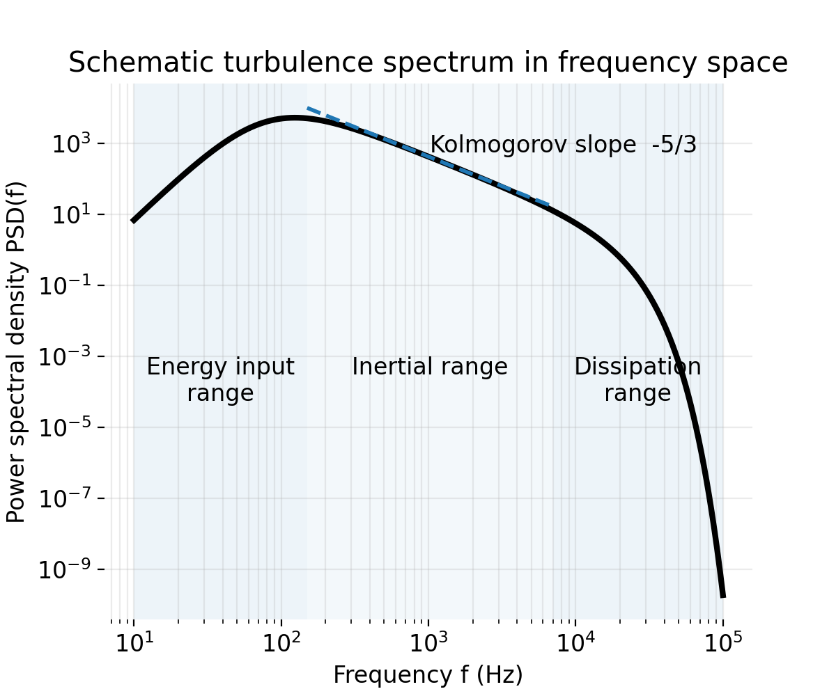
Schematic turbulence power spectrum in frequency space, illustrating the canonical separation into energy input range, inertial range, and dissipation range. At low frequencies, the spectrum rises toward a maximum that represents the energy containing scales where kinetic energy is injected into the flow. At intermediate frequencies, the spectrum follows a power law consistent with Kolmogorov’s prediction, with a slope of $-5/3$, indicating scale local energy transfer without dissipation. At high frequencies, the spectrum steepens rapidly due to viscous dissipation, where kinetic energy is converted into heat. The axes are shown on logarithmic scales, and the dashed line marks the reference $-5/3$ scaling within the inertial range

Dissipation range and the role of viscosity

The basic reason a dissipative cutoff exists is visible directly from the scaling of the viscous term. For a characteristic length scale $L$, the Laplacian scales as $\Delta \sim 1/L^2$, so the viscous term scales like

\[\underbrace{\nu \Delta \mathbf{v}}_{\text{dissipation range}} \sim \frac{\nu}{L^2}\,\mathbf{v}.\]

This immediately implies a key consequence.

As the length scale $L$ decreases, viscous effects grow as $1/L^2$.

The transition into the dissipation range occurs when the viscous term becomes comparable to the inertial term. In scaling form, this corresponds to

\[\nu \Delta \mathbf{v} \gtrsim (\mathbf{v} \cdot \nabla)\mathbf{v}.\]

In terms of wavenumber, the dissipation cutoff occurs when $k$ exceeds the inverse Kolmogorov scale,

\[k > \delta^{-1} = \left(\frac{\nu^3}{\epsilon}\right)^{-\tfrac{1}{4}}.\]

This gives the Kolmogorov scale the interpretation of the characteristic eddy size at which the dynamics transition from an inertial transfer regime to a viscous dissipation regime.

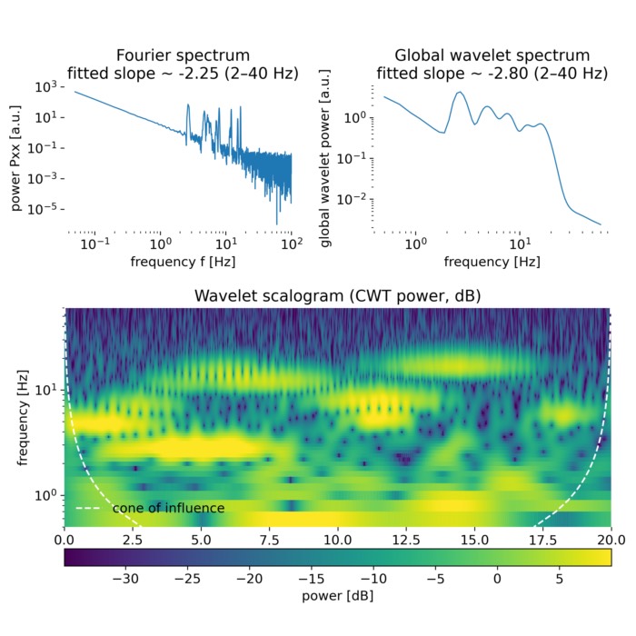
Spectral analysis of turbulence and the energy spectrum

A practical way to diagnose cascades and scaling laws in simulations is through spectral analysis. The core idea is to transform spatial fields into Fourier space, interpret Fourier modes as contributions from different length scales, and compute an isotropically averaged spectrum $E(k)$ that depends only on the wavenumber magnitude $k = \sqrt{k_x^2 + k_y^2}$.

In a periodic domain of size $L_x$ by $L_y$ discretized by $n_x$ by $n_y$ grid points, the discrete Fourier wavenumbers in each direction are

\[\begin{aligned} k_x &= 2\pi \,\mathrm{fftfreq}(n_x, d=L_x/n_x), \\ k_y &= 2\pi \,\mathrm{fftfreq}(n_y, d=L_y/n_y), \end{aligned}\]

where $\mathrm{fftfreq}$ denotes the standard discrete Fourier frequency grid. From these, a two dimensional wavenumber grid and squared magnitude are formed as

\[k^2 = k_x^2 + k_y^2.\]

In the vorticity streamfunction formulation, e.g., used in numerical simulations to enforce incompressibility and to drive the velocity field from a scalar evolved quantity, the primary evolved field is vorticity $\omega$. The streamfunction $\psi$ satisfies

\[\nabla^2 \psi = -\omega.\]

In Fourier space, with $\widehat{\psi}$ and $\widehat{\omega}$ denoting Fourier transforms, this becomes

\[-k^2 \widehat{\psi} = -\widehat{\omega} \quad\Rightarrow\quad \widehat{\psi} = \frac{\widehat{\omega}}{k^2},\]

with the convention that the mean mode $\widehat{\psi}(0,0)$ is set to zero. The incompressible velocity field is obtained from the streamfunction via

\[u = \partial_y \psi, \quad v = -\partial_x \psi,\]

so in Fourier space the velocity modes are

\[\widehat{u} = i k_y \widehat{\psi}, \quad \widehat{v} = -i k_x \widehat{\psi}.\]

The kinetic energy per Fourier mode is then proportional to $|\widehat{u}|^2 + |\widehat{v}|^2$. Up to normalization factors dependent on Fourier transform conventions, one defines a modal energy density

\[e(\mathbf{k}) = \frac12 \left(|\widehat{u}(\mathbf{k})|^2 + |\widehat{v}(\mathbf{k})|^2\right).\]

To obtain an isotropic spectrum $E(k)$, modes are grouped by their wavenumber magnitude $k = |\mathbf{k}|$ into bins, and energies in each bin are summed. If bins have width $\Delta k$, then one may define a spectral density by dividing by $\Delta k$,

\[E(k_j) \approx \frac{1}{\Delta k_j} \sum_{\mathbf{k} \in \text{bin } j} e(\mathbf{k}).\]

In practice, bins can be chosen either linearly spaced in $k$ or logarithmically spaced. Logarithmic binning is often helpful when one wants to visualize scaling behavior across many decades, because it distributes resolution more evenly in log space. A consequence is that bins at small $k$ can become sparsely populated because the number of discrete modes at very small wavenumbers is limited. A simple and transparent handling is to track the count $N_k$ of modes per bin and mark bins with zero counts as undefined, avoiding plotting artifacts.

Once an isotropic spectrum $E(k)$ has been computed, scaling laws can be tested by fitting power laws in log space. A power law

\[E(k) \propto k^{m}\]

is equivalent to

\[\log E(k) = a + m \log k.\]

Linear regression of $\log E$ on $\log k$ over a chosen wavenumber interval yields an estimated slope $m$. In inertial range analysis, the interval selection is crucial. One should avoid the forcing band, where energy injection distorts the spectrum, and avoid the dissipation range, where viscosity imposes a steep cutoff.

Forcing scale and spectral regimes in a forced simulation

In a forced turbulent simulation, the forcing introduces a characteristic wavenumber band. Denote the forcing wavenumber as $k_f$. In Fourier based forcing schemes, $k_f$ is the magnitude around which energy is injected, corresponding to a typical forcing length scale

\[\ell_f \sim \frac{2\pi}{k_f}.\]

As turbulence evolves, energy redistribution creates distinct spectral regimes. A minimal interpretation of spectra in forced turbulence distinguishes an energy containing large scale range, an inertial transfer regime, and a dissipation regime. In practice, the spectrum often shows an additional steep falloff at the highest wavenumbers set by numerical resolution and dealiasing. This high wavenumber cutoff reflects the combined effects of viscous dissipation, finite grid spacing, and spectral filtering.

A key diagnostic objective is therefore not merely to observe a straight line segment in a log log plot, but to identify an interval between forcing and dissipation where a power law is plausible and consistent across time, and where the fitted exponent is physically interpretable.

Conclusion

Turbulence emerges as a dynamical regime in which nonlinear advection couples a wide hierarchy of spatial and temporal scales, rendering detailed prediction intractable while giving rise to robust statistical structure. The Richardson cascade provides a unifying conceptual framework for this behavior by organizing turbulent motion into an energy input range, an inertial range governed by conservative scale to scale transfer, and a dissipation range where viscosity irreversibly removes kinetic energy. Kolmogorov’s phenomenological theory refines this picture by identifying universal scaling laws in the inertial range and by linking the small scale cutoff to the mean energy dissipation rate and the viscosity through simple dimensional arguments.

Spectral analysis offers a practical bridge between these ideas and concrete numerical or experimental data. By transforming velocity or vorticity fields into Fourier space and constructing isotropically averaged spectra, one can directly observe the separation of regimes, test scaling predictions such as the $k^{-5/3}$ law, and diagnose the influence of forcing, dissipation, and finite resolution. At the same time, the discussion highlights that spectra are not static objects but evolve in time, and that careful interpretation is required to distinguish genuine inertial range behavior from artifacts introduced by forcing bands, sparse mode counts at small wavenumbers, or numerical cutoffs at large wavenumbers.

In the next post, we will make these general concepts more concrete. We will turn to an explicit numerical realization of the Richardson cascade in a forced two dimensional turbulence simulation, examine how energy is injected at a prescribed forcing scale, and analyze the resulting spectra in detail. This will allow us to connect the abstract phenomenological picture developed here to actual simulation data and to discuss in a controlled setting how inertial range scaling emerges, fluctuates, and eventually breaks down.

Update and code availability: This post and its accompanying Python code were originally drafted in 2021 and archived during the migration of this website to Jekyll and Markdown. In January 2026, I substantially revised and extended the code. The updated and cleaned-up implementation is now available in this new GitHub repositoryꜛ. Please feel free to experiment with it and to share any feedback or suggestions for further improvements.

References and further reading

• Walter Greiner, Horst Stock, Hydrodynamik - Ein Lehr- und Übungsbuch; mit Beispielen und Aufgaben mit ausführlichen Lösungen, 1991, Harri Deutsch Verlag, ISBN: 9783817112043
• Heinz Schade and Ewald Kunz, Strömungslehre, 2007, de Gruyter, ISBN: 978-3-11-018972-8
• Sirovich Antman, J. E. Marsden, Hale P Holmes, J. Keller, J. Keener, B. J. Mielke, A. Matkowsky, C. S. Sreenivasan, and K. R. S. Perkin, Prandtl’s Essential of Fluid Mechanics, 2004, Vol. 158, Springer, ISBN: 0-387-40437-6
• O. G. Drazin, Introduction to hydrodynamic stability, 2002, Cambridge University Press, ISBN: 0521 80427 2
• Rutherford Aris, Vectors, tensors and the basic equations of fluid mechanics, 1962, Dover Publications Inc., ISBN: 0-486-66110-5
• Jianping Zhu, Computational Simulations and Applications, 2011, Intechweb.org, ISBN: 978-953-307-430-6
• Pieter Wesseling, Principles of computational fluid dynamics, 2001, Springer-Verlag, ISBN: 3-540-67853-0
• Franz Durst, Grundlagen der Strömungslehre, 2006, Springer-Verlag, ISBN: 978-3-540-31323-6
• Wilhelm Kley, Numerische Hydrodynamik, 2004, Universitaet Tuebingen (Lecture Notes)
• Burg, K., Haf, H., Wille, F., & Meister, A. Partielle Differentialgleichungen und funktionalanalytische Grundlagen, 2010, 5th ed., Vieweg + Teubner, ISBN: 978-3-8348-1294-0
• Lord Kelvin (William Thomson), Hydrokinetic solutions and observations, 1871, Philosophical Magazine. 42: 362–377
• Hermann von Helmholtz, Über discontinuierliche Flüssigkeits-Bewegungen [On the discontinuous movements of fluids]”, 1868, Monatsberichte der Königlichen Preussische Akademie der Wissenschaften zu Berlin. 23: 215–228
• Lewis Fry Richardson, Weather Prediction by Numerical Process, 1922, Cambridge University Press, ISBN: 9780521680448, archive.orgꜛ
• Kolmogorov, A. N., The local structure of turbulence in incompressible viscous fluid for very large Reynolds numbers, 1890, Vol. 434, No. 1890, Turbulence and Stochastic Process: Kolmogorov’s Ideas 50 Years On (Jul. 8, 1991), pp. 9-13, online PDFꜛ
• Frisch, U., Turbulence: the legacy of A. N. Kolmogorov, 1995/2010, Cambridge University Press, ISBN: 978-0521457132
• Pope, S. B., Turbulent flows, 2000, Cambridge University Press, ISBN: 978-0521598866
• Davidson, P. A., Turbulence: an introduction for scientists and engineers, 2015, Oxford University Press, ISBN: 978-0198722595