Forced 2D turbulence and Richardson cascade in a pseudospectral vorticity solver
In the previous post on turbulence, we discussed the Richardson cascade and Kolmogorov type scaling and introduced them as a phenomenological and statistical way to organize turbulent dynamics across scales. This post is a direct follow up in a concrete numerical setting. Here, we implement and run a forced two dimensional incompressible turbulence simulation in vorticity streamfunction form using a pseudospectral method, and we analyze the evolving flow using isotropic energy spectra in wavenumber space. The aim is not to claim that a small code proves a full theory of turbulence, but to show explicitly what it means, in practice, to inject energy at a prescribed forcing scale $k_f$, to observe the emergence of scale separation, and to diagnose scaling regimes and cutoffs from spectral diagnostics.
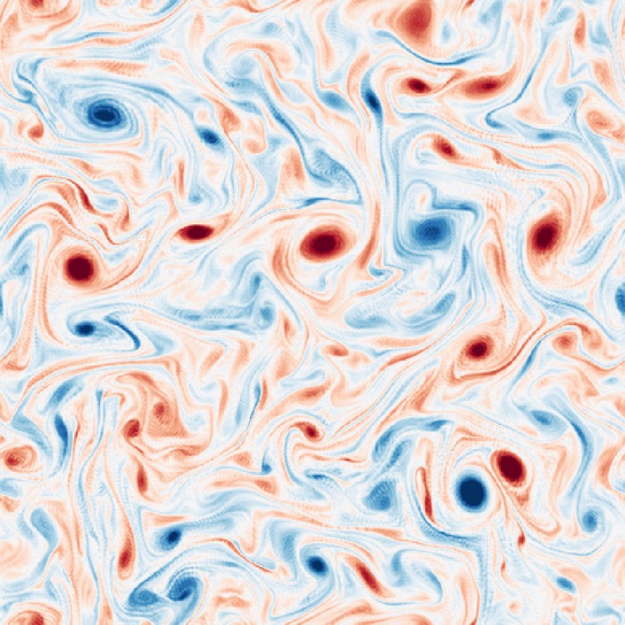
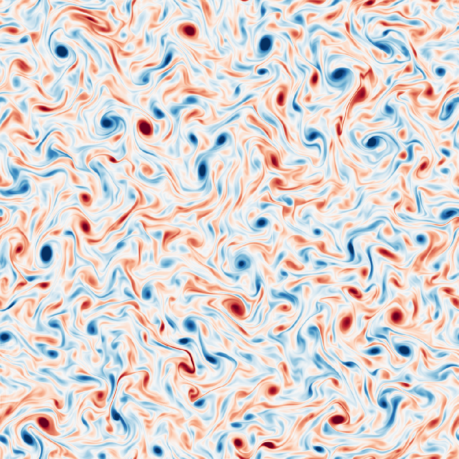
Snapshot of the vorticity field $\omega$ in the forced 2D incompressible turbulence simulation we discuss in this post. The flow is driven by stochastic forcing at intermediate wavenumbers (here: $k_f=12$), leading to the emergence of both larger scale structures through an inverse energy cascade and smaller scale filaments through a direct enstrophy cascade. The color code shows vorticity values ranging from strongly negative (blue) to strongly positive (red), with complex multiscale patterns characteristic of turbulent flows.
Mathematical background
We briefly recap the mathematical formulation from our previous post and adapt it to the present numerical experiment.
Governing equations in vorticity streamfunction form
We consider an incompressible two dimensional velocity field $\mathbf{v} = (u, v)$ on a periodic domain of size $L_x \times L_y$. Incompressibility is enforced by
\[\nabla \cdot \mathbf{v} = 0.\]Instead of evolving $\mathbf{v}$ directly, we evolve the scalar vorticity
\[\omega = \partial_x v - \partial_y u.\]In two dimensions, incompressibility allows the introduction of a streamfunction $\psi$ such that
\[u = \partial_y \psi, \quad v = -\partial_x \psi.\]The vorticity is related to $\psi$ by
\[\omega = -\nabla^2 \psi,\]so that $\psi$ can be obtained from $\omega$ by solving a Poisson equation,
\[\nabla^2 \psi = -\omega.\]The forced vorticity equation we simulate is
\[\partial_t \omega + \mathbf{v}\cdot\nabla \omega = \nu \nabla^2 \omega - \alpha \omega + f(\mathbf{x}, t).\]Here, $\nu$ is the kinematic viscosity controlling small scale dissipation, $\alpha$ is a linear drag term damping large scale energy accumulation, and $f$ is an external forcing field injecting vorticity and thus kinetic energy into the flow. In two dimensional turbulence, the presence of both $\nu$ and $\alpha$ is standard in forced simulations. Viscosity removes energy at high wavenumbers, while linear drag provides an energy sink at low wavenumbers and prevents unbounded growth of energy at the largest scales.
Fourier representation and pseudospectral method
On a periodic domain, the numerical method naturally uses Fourier expansions. Denote Fourier transforms by hats. In Fourier space, the Poisson inversion becomes algebraic:
\[\begin{aligned} & -k^2 \widehat{\psi}(\mathbf{k}) = -\widehat{\omega}(\mathbf{k})\\ \Rightarrow\quad & \widehat{\psi}(\mathbf{k}) = -\frac{\widehat{\omega}(\mathbf{k})}{k^2}, \end{aligned}\]for all $\mathbf{k}\neq 0$, and $\widehat{\psi}(\mathbf{0})$ is set to zero. From $\widehat{\psi}$, the velocity modes follow as
\[\widehat{u}(\mathbf{k}) = i k_y \widehat{\psi}(\mathbf{k}), \quad \widehat{v}(\mathbf{k}) = - i k_x \widehat{\psi}(\mathbf{k}).\]The nonlinear term $\mathbf{v}\cdot\nabla\omega$ is computed in physical space for efficiency and to avoid explicit convolutions. This defines the pseudospectral approach: compute derivatives spectrally, transform to real space, multiply, and transform back. In particular,
\[\partial_x \widehat{\omega} = i k_x \widehat{\omega}, \quad \partial_y \widehat{\omega} = i k_y \widehat{\omega}.\]Then, in physical space, compute
\[\mathbf{v}\cdot\nabla\omega = u\,\partial_x\omega + v\,\partial_y\omega,\]and transform the result back to Fourier space to obtain the spectral representation of the advective term.
Dealiasing
Quadratic nonlinearities in pseudospectral methods generate aliasing errors when modes beyond the truncation limit fold back into the represented band. A standard remedy is the two thirds rule. In this code, a rectangular two thirds mask is applied to spectral arrays, in the form
\[\widehat{g}(\mathbf{k}) \leftarrow \widehat{g}(\mathbf{k})\,M(\mathbf{k}),\]where $M(\mathbf{k})\in{0,1}$ keeps only Fourier modes satisfying $|k_x|\le k_x^{\mathrm{cut}}$ and $|k_y|\le k_y^{\mathrm{cut}}$ with $k_x^{\mathrm{cut}}\approx N_x/3$ and $k_y^{\mathrm{cut}}\approx N_y/3$ in index units. The mask is applied to the nonlinear term and to the state after each time step. This is a deliberate spectral filter. It is not intended to represent physics, but to stabilize the numerical method by preventing aliasing driven energy pile up near the grid scale.
Forcing at a prescribed wavenumber $k_f$
The simulation is forced by injecting energy in a narrow ring in wavenumber space centered at a chosen forcing magnitude $k_f$. In the code, the forcing is constructed in real space as a sum of random plane waves,
\[f(\mathbf{x}, t) = \sum_{m=1}^{N_{\mathrm{modes}}} \cos\!\big(\mathbf{k}_m\cdot \mathbf{x} + \phi_m\big),\]where each wavevector $\mathbf{k}_m$ has magnitude sampled from $[k_f(1-w),\,k_f(1+w)]$ for a relative width parameter $w$, random direction $\theta_m$, and random phase $\phi_m$. The resulting forcing field is normalized to a prescribed standard deviation and then transformed to Fourier space to enter the vorticity equation as $\widehat{f}(\mathbf{k}, t)$. The interpretation is that forcing injects energy primarily into eddies with characteristic length scale
\[\ell_f \sim \frac{2\pi}{k_f}.\]Changing $k_f$ shifts the injection scale. Larger $k_f$ corresponds to smaller forced structures.
Time stepping and CFL control
The code uses explicit second order Runge Kutta stepping in time. To maintain numerical stability, the time step is adapted using a CFL condition based on the instantaneous maximum velocity magnitude:
\[\Delta t_{\mathrm{CFL}} = c_{\mathrm{CFL}} \frac{\min(\Delta x, \Delta y)}{\max_{\mathbf{x}}\|\mathbf{v}(\mathbf{x})\|}.\]The actual time step is clipped to not exceed this bound and is also bounded below by a small floor to avoid stalling.
Isotropic energy spectrum from vorticity
A central diagnostic is the isotropically averaged kinetic energy spectrum $E(k)$ as a function of wavenumber magnitude $k=|\mathbf{k}|$. The code constructs velocity Fourier modes from $\widehat{\omega}$ via the streamfunction inversion described above, and then defines a modal kinetic energy density
\[e(\mathbf{k}) = \frac{1}{2} \Big( |\widehat{u}(\mathbf{k})|^2 + |\widehat{v}(\mathbf{k})|^2 \Big),\]up to normalization factors depending on FFT conventions. To build an isotropic spectrum, modes are grouped into bins according to $k=\sqrt{k_x^2+k_y^2}$ and energies are summed within each bin. If the $j$th bin has width $\Delta k_j$, the binned spectrum is approximated as
\[E(k_j) \approx \frac{1}{\Delta k_j} \sum_{\mathbf{k}\in \text{bin }j} e(\mathbf{k}).\]The code supports linear or logarithmic binning in $k$. Logarithmic binning is convenient when one wants to visualize scaling across multiple decades in $k$, but it introduces an important numerical reality at low $k$: very few discrete modes exist at small wavenumber magnitudes, so bins can become sparsely populated. The code therefore tracks the number of modes per bin $N_k$ and marks empty bins as undefined. This avoids spurious spikes in log log plots due to empty bins.
Finally, scaling exponents are estimated by fitting straight lines in log space over selected wavenumber intervals. For a power law $E(k)\propto k^m$, one has
\[\log E(k) = a + m \log k.\]The code performs linear regression on $(\log k, \log E)$ within the chosen fit ranges and reports the fitted slope $m$.
Numerical implementation
The implementation is organized into a compact set of functions and a main driver that runs the simulation, saves visualization frames, and produces energy spectrum plots.
The simulation state is the vorticity in Fourier space, $\widehat{\omega}$, stored as a complex array on an $n_x\times n_y$ grid. For each time step, the code constructs a forcing field in Fourier space, computes the right hand side of the vorticity equation using a pseudospectral evaluation of the nonlinear term, and advances $\widehat{\omega}$ with a second order Runge Kutta update. A dealiasing mask is applied to the nonlinear term and to the state after each update. Every fixed number of steps, the code saves a vorticity visualization in real space, computes an isotropic energy spectrum $E(k)$, and saves a log log spectrum plot with annotations including the forcing scale $k_f$ and fitted slopes in two selected wavenumber ranges.
So, let’s begin! We start by importing required libraries and setting some plotting parameters for aesthetics:
import os
import shutil
import numpy as np
import imageio.v2 as imageio
import matplotlib.pyplot as plt
from matplotlib import cm

# remove spines right and top for better aesthetics:
plt.rcParams['axes.spines.right'] = False
plt.rcParams['axes.spines.top'] = False
plt.rcParams['axes.spines.left'] = False
plt.rcParams['axes.spines.bottom'] = False
plt.rcParams.update({'font.size': 12})
Our first function we define creates 2D wavenumber grids and the squared wavenumber array:
def make_2d_wavenumbers(nx: int, ny: int, lx: float, ly: float):
    """
    Function to create 2D wavenumber grids kx, ky and squared wavenumber k2.
    """
    kx_1d = 2.0 * np.pi * np.fft.fftfreq(nx, d=lx / nx)
    ky_1d = 2.0 * np.pi * np.fft.fftfreq(ny, d=ly / ny)
    kx, ky = np.meshgrid(kx_1d, ky_1d, indexing="xy")
    k2 = kx**2 + ky**2
    return kx, ky, k2
For dealiasing, we implement the two thirds rule as follows:
def dealias_mask(nx: int, ny: int):
    """
    2/3 rule in Fourier space, rectangular mask.
    """
    kx_cut = nx // 3
    ky_cut = ny // 3
    kx_idx = np.fft.fftfreq(nx) * nx
    ky_idx = np.fft.fftfreq(ny) * ny
    kx_i, ky_i = np.meshgrid(kx_idx, ky_idx, indexing="xy")
    mask = (np.abs(kx_i) <= kx_cut) & (np.abs(ky_i) <= ky_cut)
    return mask.astype(float)
Next, we define the function to generate the stochastic ring forcing in real space and return its Fourier transform. We will need this to inject energy at a prescribed wavenumber:
def ring_forcing_realspace_hat(nx, ny, lx, ly, kf: float, width: float, nmodes: int, amp: float, rng):
    """
    Generate an isotropic stochastic real-space forcing as a sum of
    plane waves and return its 2D Fourier transform.
    """
    x = (lx / nx) * np.arange(nx)
    y = (ly / ny) * np.arange(ny)
    xx, yy = np.meshgrid(x, y, indexing="xy")

    f = np.zeros((ny, nx), dtype=np.float64)

    kmin = (1.0 - width) * kf
    kmax = (1.0 + width) * kf

    for _ in range(nmodes):
        kk = rng.uniform(kmin, kmax)
        theta = rng.uniform(0.0, 2.0 * np.pi)
        ph = rng.uniform(0.0, 2.0 * np.pi)

        kx = kk * np.cos(theta)
        ky = kk * np.sin(theta)

        f += np.cos(kx * xx + ky * yy + ph)

    f /= max(np.std(f), 1e-12)
    f *= amp

    f_hat = np.fft.fft2(f)
    f_hat[0, 0] = 0.0 + 0.0j
    return f_hat
For the Runge Kutta time stepping, we need to compute the right-hand side of the vorticity equation. This function also returns the real-space velocity components for CFL diagnostics:
def rhs_vorticity_and_uv(omega_hat, kx, ky, k2, nu: float, alpha: float, dealias: np.ndarray, f_hat):
    """
    Compute the right-hand side of the vorticity equation in Fourier space and
    return the real-space velocity components for CFL diagnostics.
    """
    psi_hat = np.zeros_like(omega_hat)
    psi_hat[k2 != 0] = -omega_hat[k2 != 0] / k2[k2 != 0]
    psi_hat[0, 0] = 0.0 + 0.0j

    u_hat = 1j * ky * psi_hat
    v_hat = -1j * kx * psi_hat

    u = np.fft.ifft2(u_hat).real
    v = np.fft.ifft2(v_hat).real

    domega_dx = np.fft.ifft2(1j * kx * omega_hat).real
    domega_dy = np.fft.ifft2(1j * ky * omega_hat).real

    adv = u * domega_dx + v * domega_dy
    adv_hat = np.fft.fft2(adv) * dealias

    diff_hat = -nu * k2 * omega_hat
    drag_hat = -alpha * omega_hat

    rhs_hat = -adv_hat + diff_hat + drag_hat + f_hat
    return rhs_hat, u, v
To compute the isotropic energy spectrum from the vorticity Fourier modes, we use the following function:
def isotropic_energy_spectrum_from_omega_hat(omega_hat, kx, ky, k2, lx, ly, nbins=120, use_log_bins=True):
    """
    Compute the isotropically averaged energy spectrum E(k) from omega_hat.
    """
    ny, nx = omega_hat.shape

    # streamfunction:
    psi_hat = np.zeros_like(omega_hat)
    psi_hat[k2 != 0] = -omega_hat[k2 != 0] / k2[k2 != 0]
    psi_hat[0, 0] = 0.0 + 0.0j

    u_hat = 1j * ky * psi_hat
    v_hat = -1j * kx * psi_hat

    norm = (1.0 / (nx * ny))**2
    e_mode = 0.5 * norm * (np.abs(u_hat)**2 + np.abs(v_hat)**2)

    k_mag = np.sqrt(k2).ravel()
    e_flat = e_mode.ravel()

    mask = k_mag > 0
    k_mag = k_mag[mask]
    e_flat = e_flat[mask]

    k_min = k_mag.min()
    k_max = k_mag.max()

    if use_log_bins:
        bins = np.logspace(np.log10(k_min), np.log10(k_max), nbins + 1)
    else:
        bins = np.linspace(k_min, k_max, nbins + 1)

    which = np.digitize(k_mag, bins) - 1
    which = np.clip(which, 0, nbins - 1)

    Ek_sum = np.bincount(which, weights=e_flat, minlength=nbins)
    N_k = np.bincount(which, minlength=nbins)

    dk = bins[1:] - bins[:-1]
    E_k = Ek_sum / np.maximum(dk, 1e-12)

    # mark empty bins as NaN so log plotting does not create spikes
    E_k[N_k == 0] = np.nan

    k_centers = 0.5 * (bins[:-1] + bins[1:])
    return k_centers, E_k, N_k
We also want to fit power law slopes to segments of the spectrum. The following function performs a linear fit in log-log space over a specified wavenumber range:
def fit_power_law_slope(k, E, k_lo, k_hi, eps=1e-30, N_k=None, min_count=0):
    k = np.asarray(k)
    E = np.asarray(E)

    mask = (k >= k_lo) & (k <= k_hi) & np.isfinite(k) & np.isfinite(E) & (E > eps)
    if N_k is not None:
        mask = mask & (np.asarray(N_k) >= min_count)

    k_use = k[mask]
    E_use = E[mask]

    if k_use.size < 5:
        return np.nan, np.nan, int(k_use.size)

    x = np.log(k_use)
    y = np.log(E_use)
    m, a = np.polyfit(x, y, 1)
    return float(m), float(a), int(k_use.size)
To visualize the spectrum and fitted slopes, we define a plotting function that saves the plot as a PNG file:
def spectrum_frame_png(
    k_centers,
    E_k,
    path,
    kf=None,
    title=None,
    # Fit options
    fit_left=True,
    fit_right=True,
    left_frac=(0.45, 1.05),    # Fit range relative to kf: [0.6*kf, 0.9*kf]
    right_frac=(1.5, 3.5),   # Fit range relative to kf: [1.2*kf, 4.0*kf]
    right_cap_frac=0.6,      # additionally: k_hi <= right_cap_frac * k_max
    eps=1e-30,
    N_k=None,):
    """
    Save spectrum as log-log plot and optionally fit exponents.

    Notes:
    * Fit ranges are by default chosen relative to kf.
    * If kf is None, no fits are performed.
    """
    k_centers = np.asarray(k_centers)
    E_k = np.asarray(E_k)

    fig = plt.figure(figsize=(6, 6), dpi=150)
    ax = plt.gca()

    #ax.loglog(k_centers, np.maximum(E_k, eps), linewidth=2)
    valid = np.isfinite(k_centers) & np.isfinite(E_k) & (E_k > eps)
    ax.loglog(k_centers[valid], E_k[valid], linewidth=2)

    ax.set_xlabel("k")
    ax.set_ylabel("E(k)")

    if title is not None:
        ax.set_title(title)

    if kf is not None:
        # plot forcing wavenumber line:
        ax.axvline(kf, linestyle="--")
        # annotate:
        ax.text(
            kf * 1.05, 10**(-10),
            f"$k_f={kf:.1f}$",
            rotation=90, verticalalignment="top", horizontalalignment="left",
            color="tab:blue")

        # plot reference -5/3 left:
        k_ref = np.linspace(0.5*kf, 0.9*kf, 50)
        # skaliere an einen Punkt der Kurve
        k0 = k_ref[0]
        E0 = np.interp(k0, k_centers, E_k)
        ax.loglog(k_ref, E0 * (k_ref / k0)**(-5/3), linestyle=":", linewidth=2,
                    c="tab:cyan", label="-5/3 ref.")

        # plot reference -3 right:
        k_ref2 = np.linspace(1.2*kf, 2.0*kf, 50)
        k0 = k_ref2[0]
        E0 = np.interp(k0, k_centers, E_k)
        ax.loglog(k_ref2, E0 * (k_ref2 / k0)**(-3), linestyle=":", linewidth=2,
                    c="tab:red", label="-3 ref.")

        k_max = float(np.max(k_centers))

        annotations = []

        # left fit (inverse energy cascade range):
        if fit_left:
            k_lo = left_frac[0] * kf
            k_hi = left_frac[1] * kf
            #mL, aL, nL = fit_power_law_slope(k_centers, E_k, k_lo, k_hi, eps=eps)
            mL, aL, nL = fit_power_law_slope(k_centers, E_k, k_lo, k_hi, eps=eps, N_k=N_k, min_count=10)
            if np.isfinite(mL):
                annotations.append(f"fit k∈[{k_lo:.1f},{k_hi:.1f}]:\nslope={mL:.2f} (N={nL})")

                # draw fit line:
                k_line = np.linspace(k_lo, k_hi, 200)
                E_line = np.exp(aL) * (k_line ** mL)
                ax.loglog(k_line, E_line, linewidth=2, c="tab:green")

        # right fit (direct enstrophy cascade range):
        if fit_right:
            k_lo = right_frac[0] * kf
            k_hi = min(right_frac[1] * kf, right_cap_frac * k_max)
            mR, aR, nR = fit_power_law_slope(k_centers, E_k, k_lo, k_hi, eps=eps)
            if np.isfinite(mR):
                annotations.append(f"fit k∈[{k_lo:.1f},{k_hi:.1f}]:\nslope={mR:.2f} (N={nR})")

                k_line = np.linspace(k_lo, k_hi, 200)
                E_line = np.exp(aR) * (k_line ** mR)
                ax.loglog(k_line, E_line, linewidth=2, c="tab:orange")

        if len(annotations) > 0:
            ax.text(
                0.02, 0.02,
                "\n".join(annotations),
                transform=ax.transAxes,
                fontsize=10,
                verticalalignment="bottom",
                horizontalalignment="left",
                #bbox=dict(boxstyle="round", alpha=0.8)
            )

    #ax.set_ylim(bottom=eps, top=10**2)
    #ax.set_ylim(bottom=10**(-28), top=10**2)
    ax.set_ylim(bottom=10**(-12), top=10**2)
    ax.grid(True, which="both", alpha=0.3)
    fig.tight_layout()
    fig.savefig(path, dpi=150)
    plt.close(fig)
The next function converts the vorticity field to an RGB image for visualization, with autoscaling based on a specified percentile:
def omega_to_rgb_autoscale(omega: np.ndarray, cmap_name: str = "RdBu_r", perc: float = 99.5):
    """
    Convert vorticity field to RGB image with autoscaling based on percentile.
    """
    vlim = np.percentile(np.abs(omega), perc)
    vlim = max(vlim, 1e-12)
    cmap = cm.get_cmap(cmap_name)
    x = np.clip(omega / vlim, -1.0, 1.0)
    x01 = 0.5 * (x + 1.0)
    rgba = cmap(x01)
    rgb = (rgba[:, :, :3] * 255.0).astype(np.uint8)
    return rgb, vlim
To visualize the vorticity field and save it as a PNG image without axes or borders, we define:
def save_png(rgb: np.ndarray, path: str):
    """
    Save RGB image as PNG without axes or borders.
    """
    fig = plt.figure(figsize=(6, 6), dpi=150)
    ax = plt.axes([0, 0, 1, 1])
    ax.axis("off")
    ax.imshow(rgb, origin="lower", interpolation="nearest")
    fig.savefig(path, dpi=150)
    plt.close(fig)
Having defined all necessary components, we can now implement the main simulation function that orchestrates the time stepping, forcing, visualization, and spectrum analysis:
def simulate_2d_cascade(
    nx=256, ny=256,
    lx=2*np.pi, ly=2*np.pi,
    nu=5e-4,
    alpha=1e-2,
    dt0=2e-3,
    cfl=0.25,
    nsteps=20000,
    frame_every=20,
    seed=1,
    forcing_kf=12.0,
    forcing_width=0.20,
    forcing_nmodes=32,
    forcing_amp=200.0,
    out_dir="frames_2d_cascade",
    gif_path="cascade_2d.gif",
    gif_path_spec="cascade_2d_spectrum.gif",
    gif_fps=30,
    clear_out_dir=True,
    left_frac=(0.45, 1.05),    # Fit range relative to kf: [0.6*kf, 0.9*kf]
    right_frac=(1.5, 3.5),   # Fit range relative to kf: [1.2*kf, 4.0*kf]
    ):

    # add forcing_kf to the out_dir name to distinguish different runs:
    out_dir = f"{out_dir}_kf{forcing_kf}"
    out_dir_frames = os.path.join(out_dir, "frames")
    gif_path = f"{gif_path}_kf{forcing_kf}.gif"
    gif_path_spec = f"{gif_path_spec}_kf{forcing_kf}.gif"

    if clear_out_dir and os.path.isdir(out_dir):
        shutil.rmtree(out_dir)
    os.makedirs(out_dir, exist_ok=True)
    os.makedirs(out_dir_frames, exist_ok=True)

    energy_dir = os.path.join(out_dir, "energy")
    os.makedirs(energy_dir, exist_ok=True)

    frames_spec = []   # RGB frames of spectrum plots for GIF

    rng = np.random.default_rng(seed)

    kx, ky, k2 = make_2d_wavenumbers(nx, ny, lx, ly)
    dealias = dealias_mask(nx, ny)

    omega0 = 0.1 * rng.standard_normal((ny, nx))
    omega_hat = np.fft.fft2(omega0) * dealias

    dx = lx / nx
    dy = ly / ny

    frames_rgb = []
    nframes = 0
    dt = float(dt0)

    for step in range(nsteps + 1):
        # step = 0
        f_hat = ring_forcing_realspace_hat(
            nx, ny, lx, ly,
            kf=forcing_kf, width=forcing_width,
            nmodes=forcing_nmodes,
            amp=forcing_amp,
            rng=rng) * dealias

        # RK2 with adaptive CFL:
        k1, u, v = rhs_vorticity_and_uv(omega_hat, kx, ky, k2, nu, alpha, dealias, f_hat)
        speed_max = float(np.max(np.sqrt(u*u + v*v)))
        dt_cfl = cfl * min(dx, dy) / max(speed_max, 1e-12)

        # limit dt to prevent jumps
        dt = min(dt, dt_cfl)
        dt = max(dt, 1e-6)

        omega_hat_mid = (omega_hat + 0.5 * dt * k1) * dealias
        k2_rhs, _, _ = rhs_vorticity_and_uv(omega_hat_mid, kx, ky, k2, nu, alpha, dealias, f_hat)
        omega_hat = (omega_hat + dt * k2_rhs) * dealias

        if step % frame_every == 0:
            omega = np.fft.ifft2(omega_hat).real
            finite = bool(np.isfinite(omega).all())
            om_rms = float(np.sqrt(np.mean(omega**2)))
            om_max = float(np.max(np.abs(omega)))

            print(f"step={step:6d} dt={dt:.3e} dt_cfl={dt_cfl:.3e} finite={finite} omega_rms={om_rms:.3e} omega_max={om_max:.3e}")

            if not finite:
                raise FloatingPointError("omega contains NaN or Inf")

            rgb, vlim = omega_to_rgb_autoscale(omega, perc=99.5)
            png_path = os.path.join(out_dir_frames, f"frame_{nframes:06d}.png")
            save_png(rgb, png_path)
            frames_rgb.append(rgb)


            # calculate and plot energy spectrum:
            k_centers, E_k, N_k = isotropic_energy_spectrum_from_omega_hat(omega_hat, kx, ky, k2, lx, ly, nbins=120)

            spec_path = os.path.join(energy_dir, f"spectrum_{nframes:06d}.png")
            spectrum_frame_png(
                k_centers, E_k,
                path=spec_path,
                kf=forcing_kf,
                title=f"Energy spectrum, frame {nframes}",
                fit_left=True,
                fit_right=True,
                left_frac=left_frac,
                right_frac=right_frac,
            )

            # load PNG as RGB frame into RAM to build a GIF at the end:
            spec_img = imageio.imread(spec_path)
            frames_spec.append(spec_img)

            nframes += 1

    imageio.mimsave(gif_path, frames_rgb, fps=gif_fps)
    print(f"Done. Wrote {nframes} frames. GIF: {gif_path}")


    imageio.mimsave(gif_path_spec, frames_spec, fps=gif_fps)
    print(f"Energy spectrum GIF saved to: {gif_path_spec}")

    return frames_rgb
To run the simulation with specified parameters, we call the main function as follows:
# %% MAIN
simulate_2d_cascade(
    nx=1024, ny=1024,         # grid points
    lx=2*np.pi, ly=2*np.pi, # domain size
    nu=1e-4,                # viscosity; start with 5e-4 for moderate, 2e-4 for weak diffusion
    alpha=5e-3,             # linear drag (friction); use: 1e-2 for moderate, 5e-3 for weak drag
    dt0=2e-3,               # initial time step
    cfl=0.25,               # CFL number for adaptive time stepping
    nsteps=20000,           # total number of time steps
    frame_every=20,         # save frame every N steps
    seed=1,                 # random seed
    forcing_kf=24.0,         # wavenumber of forcing ring; larger number leads to smaller structures; e.g., use 6 or 12
    forcing_width=0.20,     # relative width of forcing ring
    forcing_nmodes=32,      # number of random modes in forcing
    forcing_amp=200.0,      # amplitude of forcing
    out_dir="frames_2d_cascade", # output directory for frames
    gif_path="cascade_2d.gif",   # output path for GIF
    gif_path_spec="cascade_2d_spectrum.gif", # output path for spectrum GIF
    gif_fps=30,             # frames per second for GIF
    clear_out_dir=False,      # clear output directory before running
    left_frac=(0.50, 0.90),    # fit range relative to kf: [0.6*kf, 0.9*kf]
    right_frac=(1.15, 2.05),   # fit range relative to kf: [1.15*kf, 2.05*kf]
)
In summary, we used the following set of parameters:
- Grid size: 1024x1024 points
- Domain size: $2\pi \times 2\pi$
- Total time steps: 20000 (our main simulation loop runs this many steps)
- Viscosity: $\nu=1\times 10^{-4}$
- Linear drag: $\alpha=5\times 10^{-3}$ (this damps large scales)
- Initial time step: $dt_0=2\times 10^{-3}$
- CFL number: $c_{\mathrm{CFL}}=0.25$ (used to adapt time step)
- Forcing wavenumber: $k_f=24.0$ (this sets the scale at which energy is injected)
- Forcing width: 0.20 (relative width of the forcing ring in k-space)
- Number of forcing modes: 32 (number of random plane waves summed in the forcing)
- Forcing amplitude: 200.0 (scales the strength of the forcing)
Discussion of the simulation results
We now turn to the results of the two dimensional forced vorticity simulation and discuss how the evolving flow field and its energy spectrum reflect the phenomenology of the Richardson cascade as introduced in the previous post. The discussion is structured in two parts. We first consider the full temporal evolution using animated visualizations. We then analyze a sequence of representative snapshots to illustrate how spectral regimes emerge and stabilize over time.
Global temporal evolution
The full animations already convey the essential dynamics. In physical space, the initially random vorticity field quickly organizes into a dense population of interacting vortical structures. While the forcing injects energy at a fixed intermediate length scale, nonlinear advection continuously redistributes this energy both toward smaller and toward larger scales. The flow remains strongly time dependent, with ongoing vortex stretching, filament formation, and merger events.
GIFs generated by our simulation. Left: Time evolution of the vorticity field $\omega(x,y,t)$ in physical space. Right: Corresponding evolution of the isotropically averaged energy spectrum $E(k)$. Energy is injected at the forcing wavenumber $k_f=24$ and redistributed across scales by nonlinear advection. Over time, a separation between the forcing range, an inertial transfer range, and a dissipation dominated high wavenumber range becomes apparent.
In spectral space, the effect of this redistribution is seen as a progressive population of wavenumbers away from the forcing band. At early times, the spectrum is strongly peaked near $k_f$. As the simulation evolves, a broader spectral support develops and a range of wavenumbers emerges over which the spectrum approximately follows a power law. At the largest resolved wavenumbers, the spectrum steepens rapidly, reflecting viscous dissipation and the finite numerical resolution.
Initial stage: Forcing dominated regime
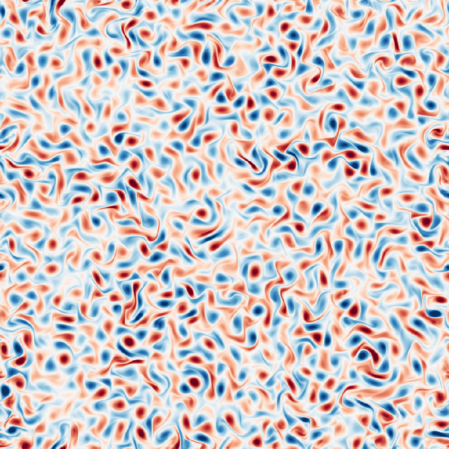
Right after initialization, the dynamics are dominated by the imposed forcing. In physical space, vortical structures are relatively small and fairly uniform in size, reflecting the narrow band of excited wavenumbers. The flow has not yet developed a clear hierarchy of scales.
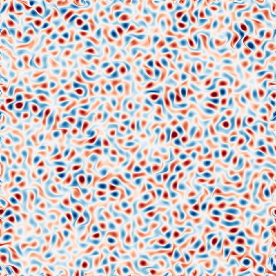
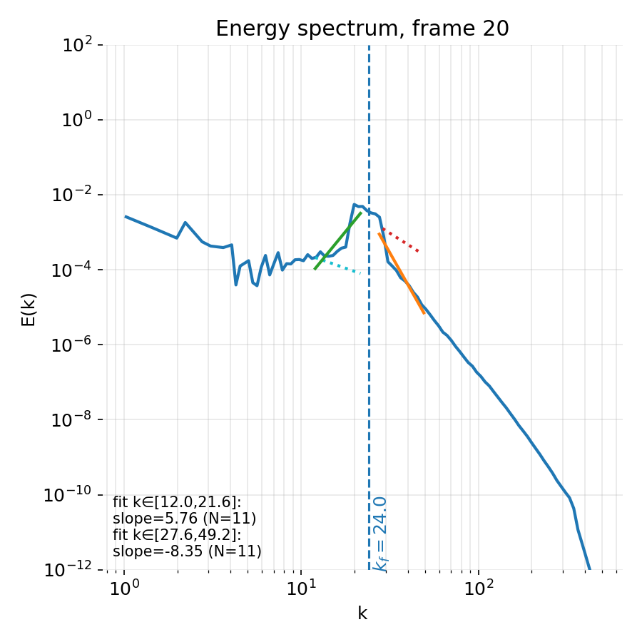
Initial stage of the simulation (frame 20). Left: Vorticity field shortly after initialization. Right: Energy spectrum dominated by the forcing scale. The spectrum is sharply peaked near $k_f$, with no extended inertial range yet established.
The energy spectrum at this stage is correspondingly narrow. Most of the energy resides close to the forcing wavenumber, and any apparent power law behavior is weak and unstable. Fits in this regime are not physically meaningful, as the cascade has not yet developed.
Early stage: Emergence of scale interaction
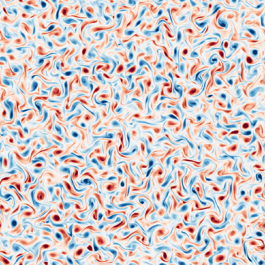
At early times, nonlinear interactions begin to redistribute energy more efficiently across scales. In physical space, this is reflected by a visibly broader distribution of vortex sizes and by the appearance of elongated filaments and vortex interactions.
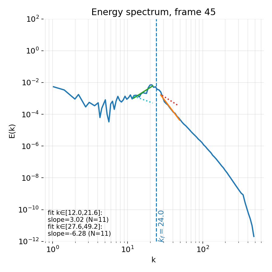
Early stage of the simulation (frame 45). Left: Increasing variability in vortex size and shape. Right: Spectral broadening around the forcing scale, with the first indications of distinct scaling behavior on either side of $k_f$.
In spectral space, the peak at the forcing wavenumber broadens and energy starts to populate both lower and higher wavenumbers. Although the spectrum is still evolving, distinct slopes begin to appear on either side of the forcing band. This marks the onset of cascade like behavior, but the inertial range is still limited in extent and the fitted exponents fluctuate strongly in time.
Developed stage: inertial transfer regime
At later times, the flow reaches a statistically stationary regime. The vorticity field displays a wide range of interacting structures, with no single characteristic scale dominating the dynamics. Large vortices coexist with fine scale filaments, consistent with the qualitative picture of the Richardson cascade.
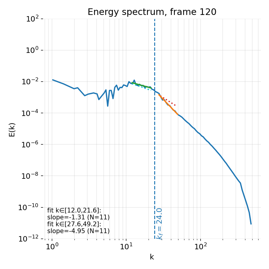
Developed turbulent state (frame 120). Left: A rich multiscale vorticity field with coexisting large and small structures. Right: Energy spectrum exhibiting a clear separation between forcing, inertial transfer, and dissipation ranges.
The corresponding energy spectrum now exhibits a well defined structure. Around the forcing scale $k_f$, energy injection is visible as a local maximum. On intermediate wavenumbers, a range emerges over which the spectrum is approximately compatible with power law scaling ($E(k) \sim k^{-5/3} \approx -1.67$ for $k < k_f$ and $E(k) \sim k^{-3}$ for $k > k_f$), consistent with the dual cascade phenomenology of two dimensional turbulence. At high wavenumbers, the spectrum steepens rapidly due to viscous dissipation. While the inertial range is limited by resolution and by the proximity of the forcing scale, its presence is robust across time.
Note, that through out the entire simulation, we never reach exact power law scaling over extended ranges. In contrast, we see the slopes fluctuate around the theoretical predictions. This is expected given the limited resolution, the finite width of the forcing band, and the ongoing time dependence of the flow. Nevertheless, the qualitative separation into forcing dominated, inertial transfer, and dissipation regimes is clear and persistent.
Late stage: Statistically steady cascade
In the late stage, both the flow field and the energy spectrum fluctuate around statistically stationary mean properties. Individual vortices continue to form, merge, and decay, but the overall distribution of scales remains stable.
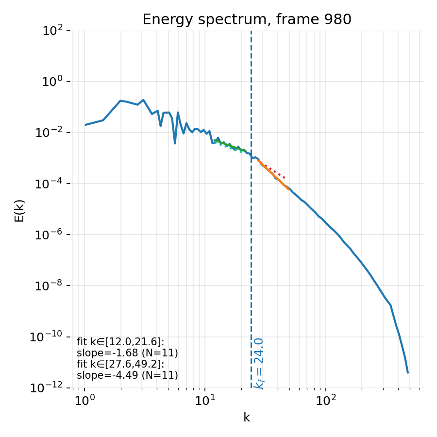
Late time snapshot in the statistically stationary regime (frame 980). Left: Persistent multiscale vorticity patterns. Right: Stabilized energy spectrum with reproducible scaling exponents and a clear dissipation cutoff.
Spectrally, the fitted slopes in the inertial transfer ranges still show temporal fluctuations. This reflects both genuine physical variability due to ongoing nonlinear interactions and statistical uncertainty arising from finite resolution and binning. Nevertheless, the qualitative separation into forcing dominated, inertial transfer, and dissipation regimes is persistent and consistent with the phenomenology of the Richardson cascade discussed earlier.
Taken together, these results demonstrate how a relatively compact spectral Navier Stokes solver, combined with controlled forcing and systematic spectral diagnostics, reproduces the central qualitative features of turbulent cascades. In the following conclusion, we summarize the main lessons from this numerical experiment and outline directions for refinement and extension.
Conclusion
In this post, we have moved from the abstract phenomenology of turbulence to a concrete numerical realization of the Richardson cascade in a controlled two dimensional setting. Building on the conceptual framework introduced in the preceding turbulence overview, we implemented and analyzed a forced incompressible Navier–Stokes solver in vorticity form, using spectral methods to resolve both the flow field and its energy distribution across scales.
The simulation demonstrates how energy injected at a prescribed forcing scale is redistributed by nonlinear advection into a multiscale flow. In physical space, this redistribution manifests as a dense and continuously evolving population of vortical structures, spanning a broad range of sizes. In spectral space, the same dynamics appear as the gradual emergence of distinct regimes: A forcing dominated range around the injection scale, an intermediate range characterized by approximately scale invariant transfer, and a dissipation dominated cutoff at high wavenumbers. While the limited resolution and finite forcing bandwidth prevent the formation of perfectly extended power law ranges, the qualitative structure of the cascade is robust and persistent over time.
An important outcome of our little experiment is, in my view, the explicit demonstration that turbulence is best understood statistically rather than instantaneously. Neither the vorticity field nor the energy spectrum settles into a static configuration. Instead, both fluctuate around statistically stationary mean properties, and fitted spectral exponents vary in time. These fluctuations are not numerical artifacts but a direct consequence of ongoing nonlinear interactions and finite size effects. This reinforces the view that power law scalings in turbulence are asymptotic statistical statements, not exact signatures observable at every instant.
From a methodological perspective, the combination of spectral time integration, controlled forcing, and isotropic spectral diagnostics provides a transparent and extensible framework for studying turbulent cascades. Our code illustrates how theoretical concepts such as forcing scales, inertial transfer, and dissipation can be mapped directly onto numerical observables. At the same time, it highlights the practical limitations imposed by resolution, dealiasing, and finite domains, which must be kept in mind when interpreting spectral fits.
In the broader context, our numerical experiment may serve as a bridge between phenomenological turbulence theory and concrete simulation practice. I think, it shows how the Richardson cascade, Kolmogorov scaling arguments, and spectral analysis come together in an explicit computational setting. This connection is valuable not only for deepening conceptual understanding but also for informing the design and interpretation of more complex simulations in geophysical, astrophysical, and engineering contexts.
Update and code availability: This post and its accompanying Python code were originally drafted in 2021 and archived during the migration of this website to Jekyll and Markdown. In January 2026, I substantially revised and extended the code. The updated and cleaned-up implementation is now available in this new GitHub repositoryꜛ. Please feel free to experiment with it and to share any feedback or suggestions for further improvements.
References and further reading
- Walter Greiner, Horst Stock, Hydrodynamik - Ein Lehr- und Übungsbuch; mit Beispielen und Aufgaben mit ausführlichen Lösungen, 1991, Harri Deutsch Verlag, ISBN: 9783817112043
- Heinz Schade and Ewald Kunz, Strömungslehre, 2007, de Gruyter, ISBN: 978-3-11-018972-8
- Sirovich Antman, J. E. Marsden, Hale P Holmes, J. Keller, J. Keener, B. J. Mielke, A. Matkowsky, C. S. Sreenivasan, and K. R. S. Perkin, Prandtl’s Essential of Fluid Mechanics, 2004, Vol. 158, Springer, ISBN: 0-387-40437-6
- O. G. Drazin, Introduction to hydrodynamic stability, 2002, Cambridge University Press, ISBN: 0521 80427 2
- Rutherford Aris, Vectors, tensors and the basic equations of fluid mechanics, 1962, Dover Publications Inc., ISBN: 0-486-66110-5
- Jianping Zhu, Computational Simulations and Applications, 2011, Intechweb.org, ISBN: 978-953-307-430-6
- Pieter Wesseling, Principles of computational fluid dynamics, 2001, Springer-Verlag, ISBN: 3-540-67853-0
- Franz Durst, Grundlagen der Strömungslehre, 2006, Springer-Verlag, ISBN: 978-3-540-31323-6
- Wilhelm Kley, Numerische Hydrodynamik, 2004, Universitaet Tuebingen (Lecture Notes)
- Burg, K., Haf, H., Wille, F., & Meister, A. Partielle Differentialgleichungen und funktionalanalytische Grundlagen, 2010, 5th ed., Vieweg + Teubner, ISBN: 978-3-8348-1294-0
- Lord Kelvin (William Thomson), Hydrokinetic solutions and observations, 1871, Philosophical Magazine. 42: 362–377
- Hermann von Helmholtz, Über discontinuierliche Flüssigkeits-Bewegungen [On the discontinuous movements of fluids]”, 1868, Monatsberichte der Königlichen Preussische Akademie der Wissenschaften zu Berlin. 23: 215–228
- Lewis Fry Richardson, Weather Prediction by Numerical Process, 1922, Cambridge University Press, ISBN: 9780521680448, archive.orgꜛ
- Kolmogorov, A. N., The local structure of turbulence in incompressible viscous fluid for very large Reynolds numbers, 1890, Vol. 434, No. 1890, Turbulence and Stochastic Process: Kolmogorov’s Ideas 50 Years On (Jul. 8, 1991), pp. 9-13, online PDFꜛ
- Frisch, U., Turbulence: the legacy of A. N. Kolmogorov, 1995/2010, Cambridge University Press, ISBN: 978-0521457132
- Pope, S. B., Turbulent flows, 2000, Cambridge University Press, ISBN: 978-0521598866
- Davidson, P. A., Turbulence: an introduction for scientists and engineers, 2015, Oxford University Press, ISBN: 978-0198722595


comments