Wavelet analysis in turbulence (and beyond)

March 18, 2021 January 28, 2026 19 minute read see also comments

Turbulent flows are intrinsically multiscale and intermittent. Energy is not only distributed across a wide range of spatial or temporal scales, but also fluctuates strongly in time. Classical Fourier based methods are well suited to quantify the global distribution of energy over scales, for example through power spectra or structure functions. However, Fourier analysis is fundamentally non-local in time: It answers the question which scales are present, but not when they are active.

Continuous wavelet transform of frequency breakdown signal. Wavelet analysis provides a joint time scale representation, allowing one to localize energetic events in both time and scale. This makes it particularly suitable for analyzing intermittent and multiscale phenomena such as turbulence (and beyond). The figure shows the wavelet power spectrum of a signal exhibiting bursts of activity at different frequencies. The color scale indicates the local energy content at each time and scale, revealing when specific frequency components are active. Source: Wikiemedia Commonsꜛ (license: public domain).

Wavelet analysis complements Fourier methods by providing a joint time scale representation. This makes it particularly suitable for turbulence, where coherent structures, bursts of activity, and intermittent events dominate the dynamics. Wavelets allow one to localize energetic events in both time and scale, to separate background fluctuations from transient structures, and to study scale dependent intermittency in a controlled and quantitative way.

In practice, wavelet analysis has become a standard tool in experimental turbulence, atmospheric and geophysical flows, space plasma turbulence, but also in neuroscience, image and signal processing, and numerical simulations, precisely because it bridges the gap between purely spectral and purely temporal descriptions.

What are wavelets and wavelet analysis

A wavelet is a localized oscillatory function with finite energy. Unlike sine and cosine functions, which extend infinitely in time, a wavelet is concentrated around a central position and decays away from it. By translating and rescaling a single prototype function, called the mother wavelet, one generates a family of functions that probe a signal at different times and different scales.

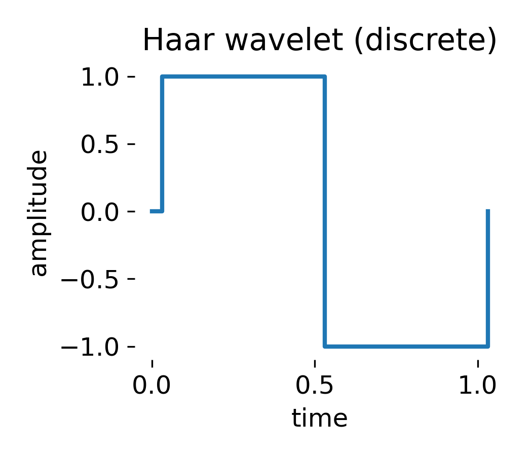
Discrete Haar wavelet shown in its standard piecewise-constant form. The Haar wavelet has compact support on the unit interval and consists of a single positive and negative step, resulting in zero mean and a single discontinuity. This structure makes the Haar wavelet particularly sensitive to sharp transitions and discontinuities in signals. It is a fundamental building block of the discrete wavelet transform and multiresolution analysis, but its lack of smoothness and continuous scalability distinguishes it clearly from wavelets used in continuous wavelet analysis. The Python script to generate this figure is available in the GitHub repository mentioned at the end of this post.

Wavelet analysis consists in projecting a signal onto this family of localized basis functions. The result is a representation that describes how strongly the signal correlates with wavelet functions of a given scale at a given time. In contrast to windowed Fourier methods, the time scale resolution adapts naturally: high frequency features are resolved with fine temporal precision, while low frequency features are resolved over longer time intervals.

From a physical perspective, wavelets can be interpreted as scale selective filters that are also localized in time. This interpretation makes them particularly intuitive for turbulence, where one often wants to identify when and at which scales energy is injected, transferred, or dissipated.

Mathematical foundations

Wavelet analysis is built upon a few key mathematical concepts. Here, we summarize the main definitions and properties relevant for applications in turbulence.

The wavelet and admissibility

Let $\psi(t)$ be a wavelet. The defining properties are

$\psi(t)$ has finite energy, $\int |\psi(t)|^2 \, dt < \infty$
$\psi(t)$ has zero mean, $\int \psi(t) \, dt = 0$

The zero mean condition ensures that the wavelet responds to fluctuations rather than constant offsets. It is closely related to the admissibility condition, which guarantees that a signal can be reconstructed from its wavelet transform.

Scaled and translated versions of the wavelet are defined as

\[\psi_{s,\tau}(t) = \frac{1}{\sqrt{s}} \, \psi\!\left(\frac{t - \tau}{s}\right)\]

where $s > 0$ is the scale parameter and $\tau$ is the translation in time. The normalization $1 / \sqrt{s}$ preserves energy across scales.

Continuous wavelet transform (CWT)

Given a real valued signal $x(t)$, its continuous wavelet transform (CWT) is defined as

\[W_x(s, \tau) = \int_{-\infty}^{\infty} x(t) \, \psi^*_{s,\tau}(t) \, dt\]

where the star denotes complex conjugation. The transform $W_x(s, \tau)$ measures the similarity between the signal and a wavelet of scale $s$ centered at time $\tau$.

For complex wavelets, such as the complex Morlet wavelet, $W_x(s, \tau)$ is complex valued. Its modulus

\[|W_x(s, \tau)|^2\]

is commonly interpreted as the wavelet power, representing the local energy content of the signal at scale $s$ and time $\tau$.

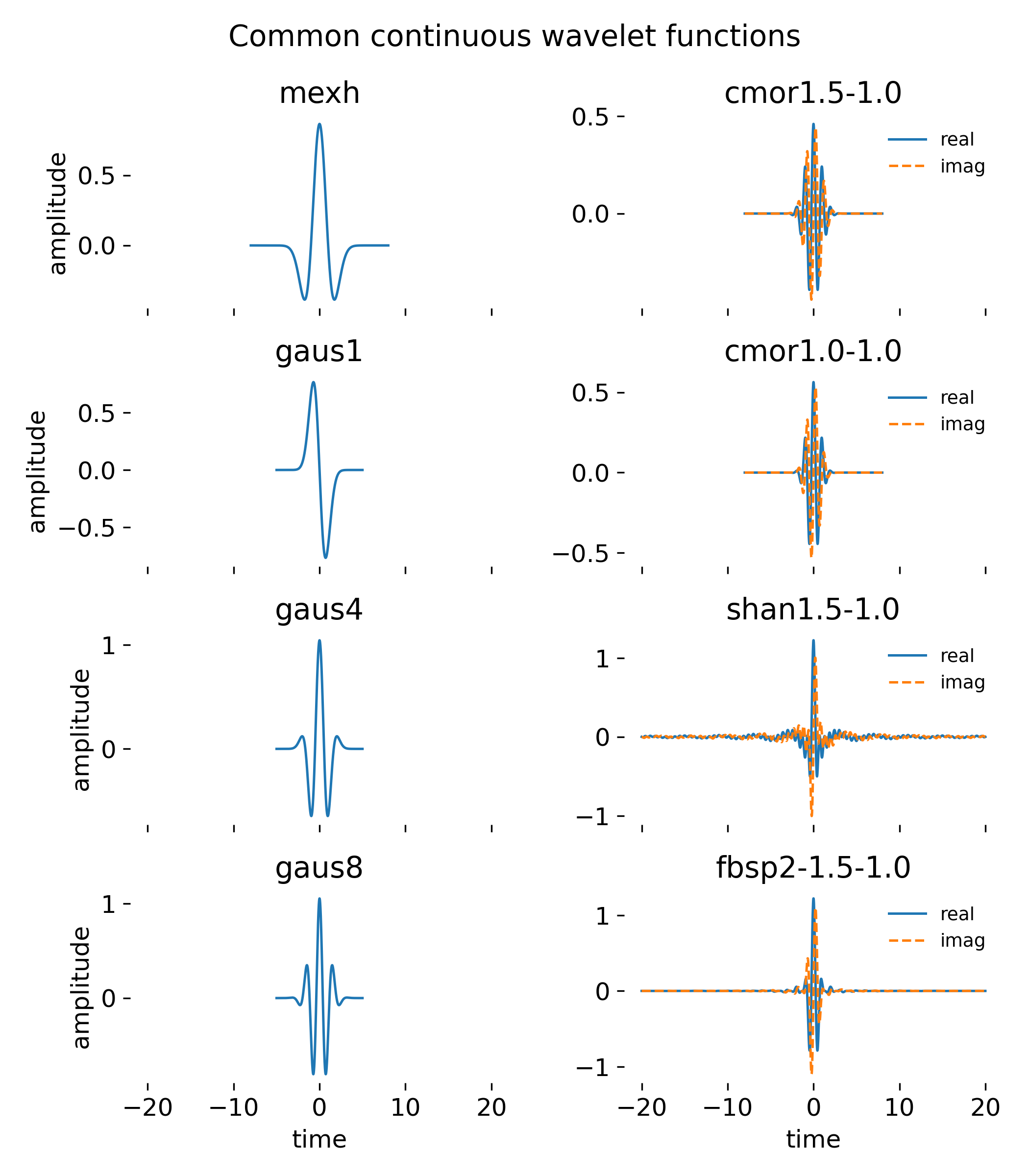
Examples of common continuous wavelet functions used in continuous wavelet analysis (CWT). The left column shows real-valued wavelets, including the Mexican hat and Gaussian wavelets of increasing order, which differ in smoothness and oscillatory structure. The right column shows complex-valued wavelets, such as Morlet, Shannon, and frequency B-spline wavelets, with real and imaginary parts plotted separately. These complex wavelets provide localized oscillatory kernels with well-defined amplitude and phase, making them particularly suitable for time–frequency analysis of nonstationary and turbulent signals. The Python script to generate this figure is available in the GitHub repository mentioned at the end of this post.

Scale and frequency (pseudo frequency)

In practice, scales are often converted to pseudo frequencies to facilitate interpretation. For a given wavelet with central frequency $f_c$, the relation between scale $s$ and frequency $f$ is approximately

\[f \approx \frac{f_c}{s}\]

up to a factor depending on the sampling interval. This mapping allows one to display wavelet power as a function of time and frequency, yielding the familiar scalogram representation.

It is important to emphasize that this frequency is not identical to Fourier frequency. It is a scale dependent quantity that reflects the dominant oscillatory content captured by the wavelet.

Global wavelet spectrum

A wavelet based analogue of the power spectrum is obtained by averaging the wavelet power over time,

\[P_\mathrm{wav}(s) = \langle |W_x(s, \tau)|^2 \rangle_\tau\]

or equivalently as a function of frequency after scale to frequency conversion. This global wavelet spectrum characterizes the average distribution of energy over scales, but retains the filtering properties of the wavelet transform. As a consequence, its scaling exponent generally differs from that obtained from a Fourier spectrum.

Cone of influence (COI)

Wavelet transforms of finite length signals suffer from edge effects, because the wavelet is no longer fully supported near the boundaries. The cone of influence (COI) defines the region in the time scale plane where these effects become significant.

For Morlet type wavelets, the cone of influence is commonly defined using the e folding time of the wavelet envelope,

\[\tau_\mathrm{COI}(s) = \sqrt{2} \, s\]

Wavelet coefficients outside this region should not be interpreted quantitatively. In visualizations, the cone of influence is typically indicated explicitly or the affected region is masked.

Numerical implementation

In numerical applications, the continuous wavelet transform is evaluated on a discrete grid of scales and times. Efficient implementations rely on convolution in the Fourier domain. In the example discussed here, a complex Morlet wavelet is used, which provides a clean separation between amplitude and phase and is well suited for energy based interpretations in turbulence.

The wavelet power is converted to logarithmic units to handle the large dynamic range characteristic of turbulent signals. Robust percentile based clipping is applied to enhance visibility of both weak and strong structures in the scalogram.

Numerical example

In the following, we illustrate wavelet analysis of a synthetic turbulence-like signal using Python. The example demonstrates how to generate a signal with a prescribed spectral exponent and intermittent bursts, compute its Fourier spectrum and continuous wavelet transform, and visualize the results.

Let’s start by importing the necessary libraries and setting up some plotting parameters:

import os
import numpy as np
import matplotlib.pyplot as plt
import pywt

RESULTS_PATH = "wavelet_analysis_figures"
os.makedirs(RESULTS_PATH, exist_ok=True)

# remove spines right and top for better aesthetics:
plt.rcParams['axes.spines.right'] = False
plt.rcParams['axes.spines.top'] = False
plt.rcParams['axes.spines.left'] = False
plt.rcParams['axes.spines.bottom'] = False
plt.rcParams.update({'font.size': 12})

The first function we generate is for creating colored noise with a specified spectral exponent:

def colored_noise(alpha: float, n: int, fs: float, rng: np.random.Generator) -> np.ndarray:
    """
    Generate 1D colored noise with power spectral density ~ 1 / f^alpha.
    alpha = 0: white noise
    alpha = 1: pink noise
    alpha = 2: brown noise

    Implementation: scale Fourier amplitudes, assign random phases, inverse FFT.
    """
    freqs = np.fft.rfftfreq(n, d=1.0 / fs)

    # amplitude ~ 1 / f^(alpha/2) so that power ~ 1 / f^alpha:
    amp = np.ones_like(freqs)
    amp[1:] = 1.0 / (freqs[1:] ** (alpha / 2.0))

    phases = rng.uniform(0.0, 2.0 * np.pi, size=freqs.shape)
    spectrum = amp * (np.cos(phases) + 1j * np.sin(phases))

    x = np.fft.irfft(spectrum, n=n)
    x = (x - x.mean()) / (x.std() + 1e-12)
    return x

Next, we define a function to add intermittent bursts of oscillations:

def intermittent_bursts(t: np.ndarray, rng: np.random.Generator, n_bursts: int = 8) -> np.ndarray:
    """
    Add intermittent, localized packets of band-limited oscillations.
    This mimics bursts where energy temporarily concentrates at specific scales.
    """
    y = np.zeros_like(t)
    T = t[-1] - t[0]

    for _ in range(n_bursts):
        t0 = rng.uniform(t[0] + 0.05 * T, t[0] + 0.95 * T)
        width = rng.uniform(0.03 * T, 0.10 * T)
        f0 = rng.uniform(1.0, 20.0)  # central frequency in Hz
        phase = rng.uniform(0.0, 2.0 * np.pi)
        amp = rng.uniform(0.8, 2.0)

        envelope = np.exp(-0.5 * ((t - t0) / width) ** 2)
        carrier = np.sin(2.0 * np.pi * f0 * (t - t0) + phase)
        y += amp * envelope * carrier

    y = (y - y.mean()) / (y.std() + 1e-12)
    return y

To compute the Fourier spectrum, we use a simple periodogram:

def periodogram(x: np.ndarray, fs: float):
    """
    Simple periodogram: |FFT|^2, one-sided.
    For real data, Welch's method is typically preferred.
    """
    n = len(x)
    X = np.fft.rfft(x)
    f = np.fft.rfftfreq(n, d=1.0 / fs)

    # normalization is sufficient for relative comparisons and slope estimation:
    Pxx = (np.abs(X) ** 2) / n
    return f, Pxx

For fitting power law slopes in log-log space, we define:

def fit_loglog_slope(f: np.ndarray, y: np.ndarray, fmin: float, fmax: float):
    """
    Linear regression in log10 space:
    log10(y) = a + b * log10(f).

    Returns the slope b.
    """
    mask = (f >= fmin) & (f <= fmax) & (y > 0) & np.isfinite(y)
    xf = np.log10(f[mask])
    yy = np.log10(y[mask])

    if len(xf) < 5:
        return np.nan, (np.nan, np.nan)

    b, a = np.polyfit(xf, yy, 1)
    return b, (a, b)

Now, we can generate the synthetic turbulence-like signal:

rng = np.random.default_rng(4)

fs = 200.0          # sampling frequency in Hz
T = 20.0            # total duration in seconds
n = int(fs * T)
t = np.arange(n) / fs

# background colored noise with spectral exponent alpha:
alpha = 5.0 / 3.0   # commonly associated with inertial-range turbulence
x_bg = colored_noise(alpha=alpha, n=n, fs=fs, rng=rng)

# add intermittent bursts:
x_b = intermittent_bursts(t, rng=rng, n_bursts=10)

# combine components and add weak white noise:
x = 0.9 * x_bg + 0.9 * x_b + 0.1 * rng.standard_normal(n)
x = (x - x.mean()) / (x.std() + 1e-12)

Next, we compute the Fourier spectrum:

f_fft, Pxx = periodogram(x, fs=fs)

# fit slope over a selected frequency band:
slope_fft, _ = fit_loglog_slope(f_fft[1:], Pxx[1:], fmin=2.0, fmax=40.0)

And finally, we perform the continuous wavelet transform and prepare for visualization:

# we use a complex Morlet wavelet for a cleaner magnitude representation. PyWavelets uses the naming scheme "cmorB-C", where:
# B controls bandwidth, C controls center frequency of the wavelet (not the signal).
wavelet = "cmor1.5-1.0"

# define frequency range for the scalogram:
fmin, fmax = 0.5, 60.0  # Hz
freqs = np.linspace(fmax, fmin, 300)  # higher resolution than before

# convert target frequencies to scales:
# for CWT in PyWavelets: f = scale2frequency(wavelet, scale) / dt
dt = 1.0 / fs
scales = pywt.frequency2scale(wavelet, freqs * dt)

coeffs, freqs_out = pywt.cwt(x, scales, wavelet, sampling_period=dt)
power = np.abs(coeffs) ** 2

# global wavelet spectrum (time-averaged power per frequency):
global_power = power.mean(axis=1)

# fit slope over the same frequency band for comparability;
slope_wav, _ = fit_loglog_slope(freqs_out, global_power, fmin=2.0, fmax=40.0)

# compute time-resolved energy in a narrow band:
band_lo, band_hi = 0.5, 0.6  # Hz, adjust as needed
band_mask = (freqs_out >= band_lo) & (freqs_out <= band_hi)
band_energy_t = power[band_mask, :].mean(axis=0)

# use log-power (dB) and robust color limits for clearer scalograms:
power_db = 10.0 * np.log10(power + 1e-12)

# robust clipping to improve contrast;
vmin = np.percentile(power_db, 5.0)
vmax = np.percentile(power_db, 99.5)

Then, we calculate the cone of influence:

# for the Morlet wavelet, the e-folding time is sqrt(2) * scale:
coi_time = np.sqrt(2.0) * scales * dt  # in seconds

t_start = t[0]
t_end = t[-1]

# left and right COI boundaries:
coi_left = t_start + coi_time
coi_right = t_end - coi_time

Finally, we create the plots.

fig = plt.figure(figsize=(9, 11))
# use GridSpec for flexible layout:
gs = fig.add_gridspec(
    nrows=3,
    ncols=2,
    height_ratios=[1.0, 1.0, 1.5],
    hspace=0.45,
    wspace=0.30)

t_min = t[0]
t_max = 20#t[-1]

# top row: signal (full width):
ax_signal = fig.add_subplot(gs[0, :])
ax_signal.plot(t, x, linewidth=1.0)
ax_signal.set_xlabel("time [s]")
ax_signal.set_ylabel("x(t) [a.u.]")
ax_signal.set_title("Synthetic intermittent turbulence-like signal")
ax_signal.set_xlim(t_min, t_max)

# middle row: Fourier spectrum (left):
ax_fft = fig.add_subplot(gs[1, 0])
ax_fft.loglog(f_fft[1:], Pxx[1:], linewidth=1.0)
ax_fft.set_xlabel("frequency f [Hz]")
ax_fft.set_ylabel("power Pxx [a.u.]")
ax_fft.set_title(f"Fourier spectrum\nfitted slope ~ {slope_fft:.2f} (2–40 Hz)")

# middle row: global wavelet spectrum (right):
ax_wav = fig.add_subplot(gs[1, 1])
ax_wav.loglog(freqs_out, global_power, linewidth=1.0)
ax_wav.set_xlabel("frequency [Hz]")
ax_wav.set_ylabel("global wavelet power [a.u.]")
ax_wav.set_title(f"Global wavelet spectrum\nfitted slope ~ {slope_wav:.2f} (2–40 Hz)")

# bottom row: wavelet scalogram (full width):
ax_sca = fig.add_subplot(gs[2, :])
extent = [t[0], t[-1], freqs_out[-1], freqs_out[0]]
im = ax_sca.imshow(
    power_db,
    aspect="auto",
    extent=extent,
    interpolation="nearest",
    vmin=vmin,
    vmax=vmax)
ax_sca.set_xlim(t_min, t_max)
ax_sca.set_yscale("log")
ax_sca.set_xlabel("time [s]")
ax_sca.set_ylabel("frequency [Hz]")
ax_sca.set_title("Wavelet scalogram (CWT power, dB)")
# overlay cone of influence:
ax_sca.plot(coi_left, freqs_out, "w--", linewidth=1.5, label="cone of influence")
ax_sca.plot(coi_right, freqs_out, "w--", linewidth=1.5)
ax_sca.legend(loc="lower left", frameon=False)
# create a new axes below the scalogram for a horizontal colorbar:
cax = fig.add_axes([
    ax_sca.get_position().x0,        # left aligned with scalogram
    ax_sca.get_position().y0 - 0.045, # slightly below scalogram
    ax_sca.get_position().width,     # same width as scalogram
    0.02                              # height of colorbar
])
cbar = fig.colorbar(im, cax=cax, orientation="horizontal")
cbar.set_label("power [dB]")

# finalize and save:
fig.tight_layout()
fig.savefig(os.path.join(RESULTS_PATH, "wavelet_analysis_overview.png"), dpi=300)
plt.close(fig)

# plot time-resolved band energy as a separate figure:
plt.figure(figsize=(12, 3.0))
plt.plot(t, band_energy_t, linewidth=1.0)
plt.xlabel("time [s]")
plt.ylabel("band energy [a.u.]")
plt.title(f"Time-resolved wavelet energy ({band_lo:.2f} to {band_hi:.2f} Hz)")
plt.tight_layout()
plt.savefig(os.path.join(RESULTS_PATH, "wavelet_analysis_band_energy.png"), dpi=300)
plt.close()

Discussion of the example

The numerical example illustrates how wavelet analysis complements classical Fourier methods when analyzing a turbulent, intermittent signal. The synthetic signal was constructed to mimic key qualitative features of turbulence: broadband spectral content, strong temporal variability, and localized bursts of activity. While it does not represent a fully developed turbulent cascade in a strict physical sense, it is sufficiently rich to demonstrate the strengths and limitations of wavelet-based analysis.

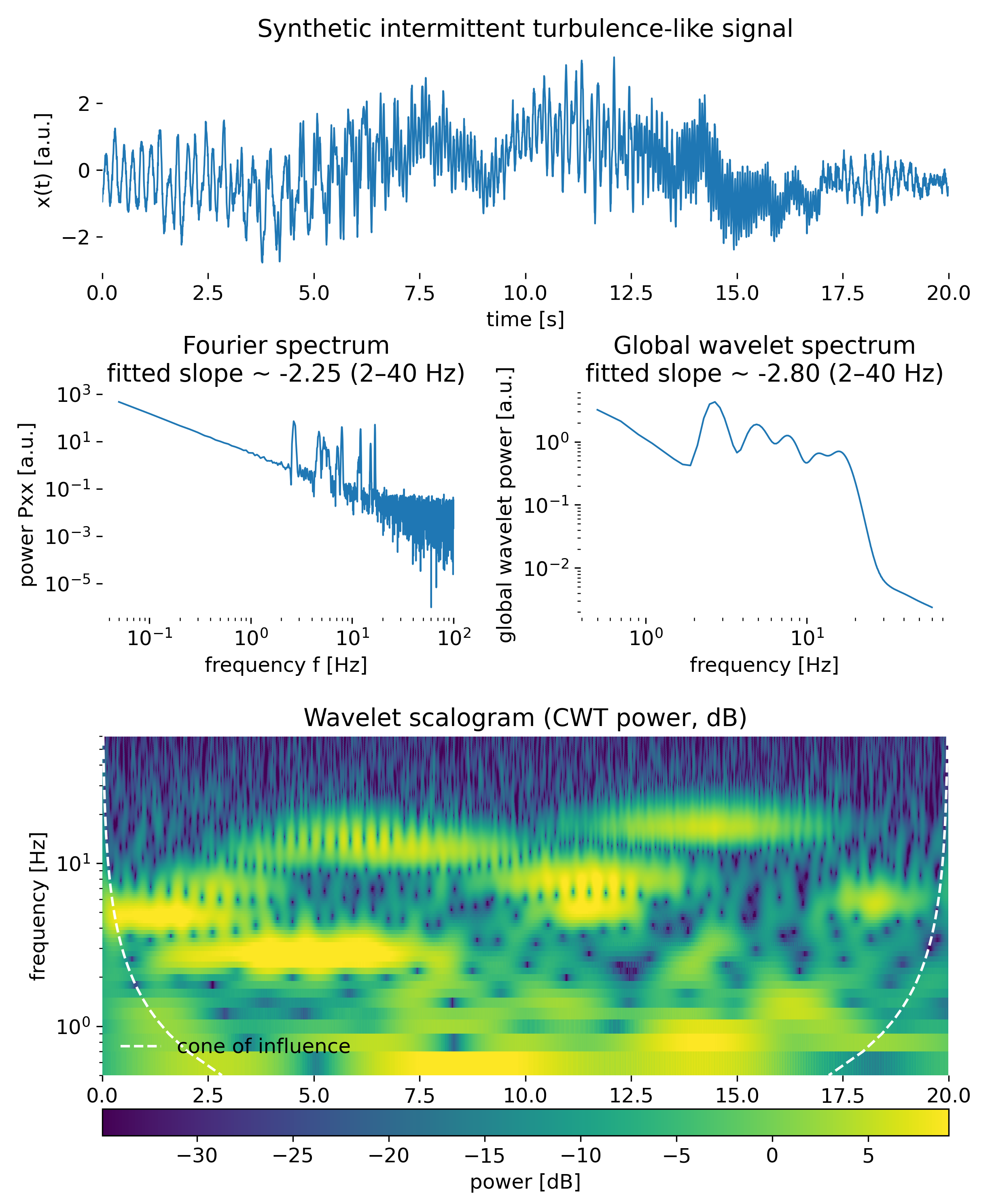
Overview of the wavelet analysis applied to a synthetic intermittent turbulence-like signal. The top panel shows the time series, illustrating strong nonstationarity and amplitude fluctuations. The middle panels compare the global Fourier power spectrum (left) and the global wavelet spectrum (right), both exhibiting approximate power-law behavior over an intermediate frequency range, but with different fitted slopes due to the distinct filtering properties of the two methods. The bottom panel shows the wavelet scalogram in logarithmic power units, revealing the temporal localization of energy across scales. The dashed curves indicate the cone of influence (COI), outside of which wavelet coefficients are affected by edge effects and should not be interpreted quantitatively.

The top panel of the overview figure shows the time series itself. Even at this level, the signal exhibits clear nonstationarity. Oscillatory components of different characteristic frequencies appear and disappear over time, and the amplitude fluctuates strongly. From the time series alone, however, it is difficult to determine which scales dominate at which times, or how these scales relate to the global spectral properties of the signal.

The Fourier spectrum, shown in the lower left panel of the overview figure, provides a global characterization of the signal. The approximate power-law decay over an intermediate frequency range indicates scale-free behavior, and the fitted slope quantifies this behavior in a compact way. At the same time, the Fourier spectrum contains no information about temporal localization. All intermittent bursts and coherent structures contribute equally to the spectrum, regardless of when they occur. In this sense, the Fourier spectrum answers the question of which scales are present on average, but not when they are active.

The global wavelet spectrum, shown in the lower right panel, plays a similar but not identical role. It is obtained by averaging the wavelet power over time and thus reflects the scale-dependent energy content of the signal filtered through the wavelet transform. The resulting slope differs from that of the Fourier spectrum, which is expected. The wavelet transform introduces scale-dependent bandwidth and localization properties, and the global wavelet spectrum should therefore not be interpreted as a direct substitute for a Fourier energy spectrum. Instead, it provides a wavelet-consistent measure of scale-dependent activity that remains sensitive to the chosen wavelet.

The most informative representation is the wavelet scalogram in the bottom panel of the overview figure. This time–frequency representation reveals how energy is distributed simultaneously in time and scale. Distinct bands of enhanced power appear at different frequencies and times, corresponding to intermittent events in the signal. These structures are not artifacts of the visualization, but reflect genuine correlations between the signal and wavelets of specific scales localized in time. The cone of influence (COI), indicated by the dashed curves, marks the region where edge effects become significant due to the finite length of the signal. Power outside this region should not be interpreted quantitatively, especially at low frequencies where the wavelet support extends over long time intervals.

Taken together, the overview figure demonstrates the central advantage of wavelet analysis for turbulent signals. While the Fourier and global wavelet spectra provide complementary global summaries, the scalogram exposes the intermittent nature of the dynamics. Energetic events are confined to specific time intervals and frequency bands, rather than being uniformly distributed over time. This is precisely the type of information that is inaccessible to purely spectral methods.

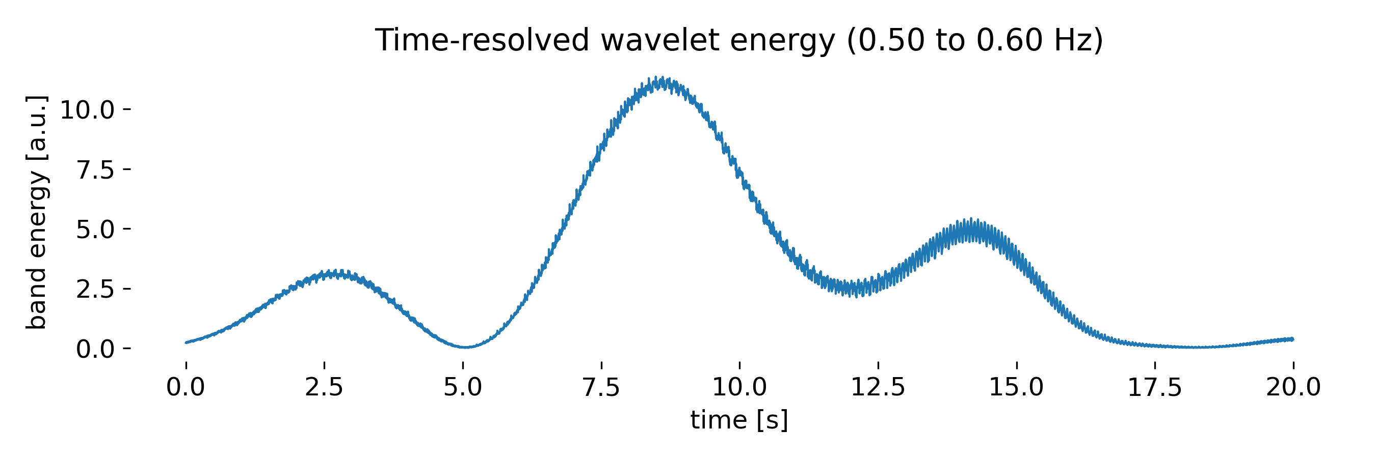
Time-resolved wavelet energy obtained by averaging the wavelet power over a narrow frequency band. The resulting curve highlights intermittent bursts of activity at the selected scale and provides a compact representation of scale-specific temporal variability. Peaks in the band energy correspond to localized regions of enhanced power in the wavelet scalogram, demonstrating how wavelet-based diagnostics can isolate and quantify intermittent dynamics.

The second figure focuses on a derived quantity: The time-resolved wavelet energy within a narrow frequency band. By averaging the wavelet power over a small frequency interval, one obtains a scalar time series that tracks the temporal modulation of energy at that scale. The resulting curve highlights periods of enhanced activity and quiescence in a way that is directly interpretable. Peaks in the band energy correspond to intervals where the scalogram shows strong power concentration in the selected frequency range. This representation is particularly useful for quantifying intermittency, detecting events, or correlating scale-specific activity with external parameters or flow features.

It is important to emphasize that such band-limited wavelet energies depend on the choice of wavelet, frequency band, and averaging procedure. They are therefore not universal quantities, but analysis tools whose meaning must be interpreted in the context of the chosen representation. When used consistently, however, they provide a powerful means of reducing complex time–frequency information to physically interpretable diagnostics.

Overall, the example illustrates how wavelet analysis extends the classical toolbox of turbulence analysis. Fourier methods remain indispensable for characterizing global scaling behavior, but wavelets add the crucial dimension of temporal localization. In turbulent and strongly nonstationary systems, this additional information is often essential for understanding the underlying dynamics.

Conclusion

Wavelet analysis provides a powerful and conceptually clear framework for studying turbulence beyond classical spectral methods. By resolving fluctuations simultaneously in time and scale, it reveals intermittent dynamics, coherent structures, and scale dependent activity that remain hidden in global Fourier representations.

At the same time, wavelet based quantities must be interpreted with care. The global wavelet spectrum is not identical to a Fourier energy spectrum, edge effects impose limits through the cone of influence, and quantitative scaling exponents depend on the chosen wavelet. When these aspects are taken into account, wavelet analysis becomes an indispensable complement to Fourier based tools in the analysis of turbulent flows.

Used judiciously, wavelets allow us to connect physical intuition about multiscale structures with mathematically controlled signal analysis, making them particularly well suited for modern experimental and numerical research in many fields of science and engineering.

Update and code availability: This post and its accompanying Python code were originally drafted in 2021 and archived during the migration of this website to Jekyll and Markdown. In January 2026, I substantially revised and extended the code. The updated and cleaned-up implementation is now available in this new GitHub repositoryꜛ. Please feel free to experiment with it and to share any feedback or suggestions for further improvements.

References and further reading

Mallat, S.A Wavelet Tour of Signal Processing, 2008, Academic Press. ISBN: 978-0123743701
Daubechies, I., Ten Lectures on Wavelets, 1992 SIAM. ISBN: 978-0898712742
Kaiser, G., A Friendly Guide to Wavelets, 1994, Birkhäuser. ISBN: 978-0817637914
Oppenheim, A. V. & Schafer, R. W., Discrete-Time Signal Processing, 2009 Pearson. ISBN: 978-0131988422
Hans-Georg Stark, Wavelets and Signal Processing: An Application-Based Introduction, 2005, Springer Berlin Heidelberg, ISBN: 3-540-23433-0
Alfred Karl Louis, Peter Maaß, and Andreas Rieder, Wavelets, Theorie und Anwendungen, 1998, Teubner, ISBN: 13:978-3-519-12094-0
Silvia Bacchelli, Serena Papi, 2006, Image denoising using principal component analysis in the wavelet domain, Journal of Computational and Applied Mathematic, Volume 189, Issues 1–2, Pages 606-621, ISSN 0377-0427, DOI: 10.1016/j.cam.2005.04.030ꜛ
Walter Greiner, Horst Stock, Hydrodynamik - Ein Lehr- und Übungsbuch; mit Beispielen und Aufgaben mit ausführlichen Lösungen, 1991, Harri Deutsch Verlag, ISBN: 9783817112043
Heinz Schade and Ewald Kunz, Strömungslehre, 2007, de Gruyter, ISBN: 978-3-11-018972-8
Sirovich Antman, J. E. Marsden, Hale P Holmes, J. Keller, J. Keener, B. J. Mielke, A. Matkowsky, C. S. Sreenivasan, and K. R. S. Perkin, Prandtl’s Essential of Fluid Mechanics, 2004, Vol. 158, Springer, ISBN: 0-387-40437-6
O. G. Drazin, Introduction to hydrodynamic stability, 2002, Cambridge University Press, ISBN: 0521 80427 2
Rutherford Aris, Vectors, tensors and the basic equations of fluid mechanics, 1962, Dover Publications Inc., ISBN: 0-486-66110-5
Jianping Zhu, Computational Simulations and Applications, 2011, Intechweb.org, ISBN: 978-953-307-430-6
Pieter Wesseling, Principles of computational fluid dynamics, 2001, Springer-Verlag, ISBN: 3-540-67853-0
Franz Durst, Grundlagen der Strömungslehre, 2006, Springer-Verlag, ISBN: 978-3-540-31323-6
Wilhelm Kley, Numerische Hydrodynamik, 2004, Universitaet Tuebingen (Lecture Notes)
Burg, K., Haf, H., Wille, F., & Meister, A. Partielle Differentialgleichungen und funktionalanalytische Grundlagen, 2010, 5th ed., Vieweg + Teubner, ISBN: 978-3-8348-1294-0
Lord Kelvin (William Thomson), Hydrokinetic solutions and observations, 1871, Philosophical Magazine. 42: 362–377
Hermann von Helmholtz, Über discontinuierliche Flüssigkeits-Bewegungen [On the discontinuous movements of fluids]”, 1868, Monatsberichte der Königlichen Preussische Akademie der Wissenschaften zu Berlin. 23: 215–228
Lewis Fry Richardson, Weather Prediction by Numerical Process, 1922, Cambridge University Press, ISBN: 9780521680448, archive.orgꜛ
Kolmogorov, A. N., The local structure of turbulence in incompressible viscous fluid for very large Reynolds numbers, 1890, Vol. 434, No. 1890, Turbulence and Stochastic Process: Kolmogorov’s Ideas 50 Years On (Jul. 8, 1991), pp. 9-13, online PDFꜛ
Frisch, U., Turbulence: the legacy of A. N. Kolmogorov, 1995/2010, Cambridge University Press, ISBN: 978-0521457132
Pope, S. B., Turbulent flows, 2000, Cambridge University Press, ISBN: 978-0521598866
Davidson, P. A., Turbulence: an introduction for scientists and engineers, 2015, Oxford University Press, ISBN: 978-0198722595