Atmosphere and ocean as hydrostatic fluids

Although atmospheric physics is today a well established and highly specialized research field, much of its conceptual and mathematical foundation belongs to classical fluid dynamics. From a physical point of view, the Earth’s atmosphere is simply a fluid under gravity. Its composition, compressibility, and thermodynamic properties introduce important specific features, but the governing principles remain those of continuum mechanics.

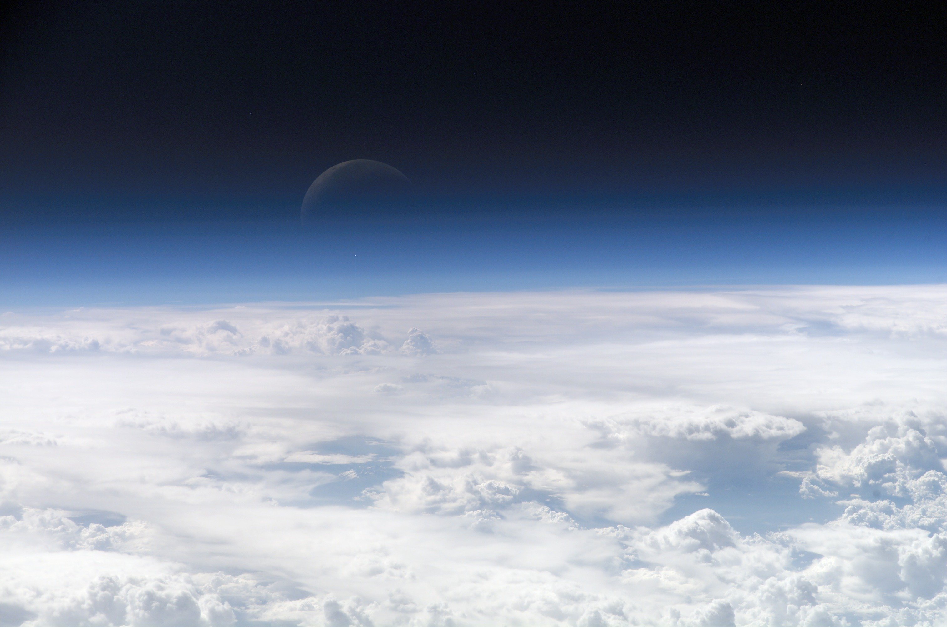
Earth’s atmosphere, photographed from the ISS (2013). Source: Wikiemedia Commonsꜛ (license: public domain).

In this post, we develop simple hydrostatic models for the vertical structure of the atmosphere and ocean.

The atmosphere is treated as a one dimensional, static fluid column in hydrostatic equilibrium. This allows the vertical structure of pressure, density, and temperature to be derived from first principles. Such models are not meant to describe weather, turbulence, or circulation, but they provide essential reference states that underlie more complex theories.

To complete the picture, an analogous hydrostatic description is developed for the ocean. The ocean differs fundamentally from the atmosphere in its equation of state and its weak compressibility, yet the same hydrostatic balance governs its vertical structure.

By placing both systems side by side, the common fluid dynamical core becomes apparent, as well as the physical reasons for their differences.

The hydrostatic atmosphere

The atmospheric model considered here is intentionally minimal. It follows 1976 work by U.S. Standard Atmosphere Committee, which established a widely used reference atmosphere for engineering applications.

The following assumptions are made:

• The atmosphere is at rest and horizontally homogeneous.
• All quantities depend only on height.
• The atmosphere is in hydrostatic equilibrium.
• Air behaves as a dry ideal gas.
• Gravity is constant with height.
• The temperature profile is prescribed.

These assumptions define a static reference atmosphere. While real atmospheres exhibit strong horizontal and temporal variability, this framework captures the dominant vertical force balance on large scales.

Hydrostatic equilibrium

Consider a thin horizontal slab of air at height $h$ with thickness $\mathrm{d}h$. Force balance in the vertical direction requires that the pressure gradient force balances gravity,

\[\frac{\mathrm{d}p}{\mathrm{d}h} = - \rho(h)\, g ,\]

where $p(h)$ is pressure, $\rho(h)$ is mass density, and $g$ is gravitational acceleration.

This equation expresses the intuitive fact that pressure decreases with height because less fluid mass overlies higher levels.

Equation of state

For dry air, the ideal gas law provides a closure relation,

\[p = \rho R T ,\]

where $T(h)$ is temperature and $R$ is the specific gas constant of dry air.

Eliminating density between the two equations yields a first order differential equation for pressure alone,

\[\frac{\mathrm{d}p}{\mathrm{d}h} = - \frac{p g}{R T(h)} .\]

At this stage, the vertical structure of the atmosphere is fully determined once the temperature profile is specified.

Prescribed temperature profile

In practice, the atmosphere is divided into layers in which the temperature varies approximately linearly with height. Within such a layer,

\[T(h) = T_b + L (h - h_b) ,\]

where $T_b$ is the temperature at the base height $h_b$, and $L$ is the lapse rate.

This piecewise linear representation captures the essential structure of the troposphere, stratosphere, and mesosphere and forms the basis of standard reference atmospheres.

Analytical pressure profiles

For a constant lapse rate $L \neq 0$, the hydrostatic equation admits the analytical solution

\[p(h) = p_b \left( \frac{T(h)}{T_b} \right)^{-\frac{g}{R L}} .\]

In isothermal layers, where $L = 0$, the solution reduces to the familiar exponential form,

\[p(h) = p_b \exp\left( -\frac{g (h - h_b)}{R T_b} \right) .\]

The density profile follows directly from the ideal gas law,

\[\rho(h) = \frac{p(h)}{R T(h)} .\]

These expressions define a complete hydrostatic atmosphere once the base conditions at sea level are specified.

The hydrostatic ocean

The ocean can also be treated as a fluid column in hydrostatic equilibrium, but important physical differences arise:

• Seawater is nearly incompressible.
• Density depends strongly on temperature and salinity.
• Pressure dependence of density cannot be neglected at depth.
• The equation of state is nonlinear and empirically constrained.

Despite these differences, the vertical force balance remains governed by hydrostatics.

Hydrostatic balance in the ocean

Using depth $z$ measured positively downward from the surface, hydrostatic equilibrium takes the form

\[\frac{\mathrm{d}p}{\mathrm{d}z} = \rho(z)\, g .\]

The sign difference compared to the atmosphere arises purely from the coordinate convention.

Equation of state for seawater

Unlike air, seawater cannot be described by a simple ideal gas law. Instead, density is a function of salinity, temperature, and pressure,

\[\rho = \rho(S, T, p) .\]

In modern physical oceanography, this relation is given by the TEOS 10 standard, which is based on the Gibbs free energy of seawater. It provides thermodynamically consistent expressions for in situ density and related quantities.

This dependence introduces a coupling between pressure and density that is absent in the atmospheric case.

Implicit structure of the hydrostatic equation

Substituting the seawater equation of state into the hydrostatic balance yields an implicit problem,

\[\frac{\mathrm{d}p}{\mathrm{d}z} = g\, \rho\big(S(z), T(z), p(z)\big).\]

Because pressure appears on both sides of the equation, no closed analytical solution exists in general. Instead, the vertical pressure profile must be obtained numerically.

Numerical solution strategy

A convenient and robust approach is fixed point iteration:

1. Prescribe temperature and salinity profiles as functions of depth.
2. Initialize the pressure using a constant density approximation.
3. Compute density from the current pressure estimate.
4. Integrate the hydrostatic equation to update pressure.
5. Iterate until convergence.

For a one dimensional column, this procedure converges rapidly and yields physically consistent pressure and density profiles.

Numerical examples

As a practical demonstration, we implement the hydrostatic atmosphere model in Python. The code computes vertical profiles of temperature, pressure, and density (and salinity) for both the atmosphere and ocean.

Numerical atmosphere profile

In the script below, the vertical coordinate is discretized, and the temperature profile is specified piecewise according to standard lapse rates. Within each layer, pressure is computed analytically using the appropriate hydrostatic solution. The base pressure and temperature are passed consistently from one layer to the next.

Density is then obtained directly from the ideal gas law. Because the governing equations are solved analytically within each layer, numerical errors are minimal and arise primarily from the discretization of the vertical coordinate.

Let’s begin by importing necessary libraries and setting up some plotting parameters:

import os
import numpy as np
import matplotlib.pyplot as plt

# remove spines right and top for better aesthetics:
plt.rcParams['axes.spines.right'] = False
plt.rcParams['axes.spines.top'] = False
plt.rcParams['axes.spines.left'] = False
plt.rcParams['axes.spines.bottom'] = False
plt.rcParams.update({'font.size': 12})

We first define physical constants and base conditions for the atmosphere: We choose a standard gravitational acceleration and the specific gas constant for dry air. Sea level conditions are set to standard temperature and pressure values:

# %% CONSTANTS AND BASE CONDITIONS
# physical constants (standard):
g0 = 9.80665            # m/s^2
R  = 287.05287          # J/(kg K), specific gas constant for dry air

# sea level base conditions:
T0 = 288.15             # K
p0 = 101325.0           # Pa

RESULTS_PATH = "hydrostatic_atmosphere_1D_figures"
os.makedirs(RESULTS_PATH, exist_ok=True)

This is our main function to compute the atmospheric profiles given an array of altitudes in meters. It handles multiple layers with different lapse rates and computes temperature, pressure, and density accordingly. It integrates layer by layer, ensuring continuity at layer boundaries:

def standard_atmosphere_1d(h_m: np.ndarray) -> tuple[np.ndarray, np.ndarray, np.ndarray]:
    """
    Compute T(h), p(h), rho(h) for altitudes h_m (meters).

    Parameters
    ----------
    h_m : array_like
        Altitudes in meters. Must be >= 0.

    Returns
    -------
    T : np.ndarray
        Temperature in K.
    p : np.ndarray
        Pressure in Pa.
    rho : np.ndarray
        Density in kg/m^3.
    """
    h_m = np.asarray(h_m, dtype=float)
    if np.any(h_m < 0):
        raise ValueError("Altitudes must be >= 0 m.")

    # Layer definition: base altitude hb [m], top altitude ht [m], lapse rate L [K/m]
    # L = dT/dh (positive means temperature increases with altitude).
    layers = [
        (0e3,   11e3,  -6.5e-3),   # Troposphere
        (11e3,  20e3,   0.0),      # Tropopause region (isothermal)
        (20e3,  32e3,  +1.0e-3),   # Stratosphere (1)
        (32e3,  47e3,  +2.8e-3),   # Stratosphere (2)
        (47e3,  51e3,   0.0),      # Stratopause region (isothermal)
        (51e3,  71e3,  -2.8e-3),   # Mesosphere (1)
        (71e3,  86e3,  -2.0e-3),   # Mesosphere (2)
    ]

    # prepare outputs:
    T = np.empty_like(h_m)
    p = np.empty_like(h_m)

    # we compute layer by layer, keeping base conditions (Tb, pb) consistent.
    Tb = T0
    pb = p0
    hb_prev = 0.0

    # helper: advance base conditions to a new base altitude by integrating through layers;
    # in this implementation we do it naturally while looping over layers:

    for hb, ht, L in layers:
        # If we skipped something (should not happen), ensure consistency
        if hb != hb_prev:
            raise RuntimeError("Layer bases are not contiguous. Check layer list.")

        # Mask of points in this layer
        mask = (h_m >= hb) & (h_m <= ht)
        h = h_m[mask]

        # temperature profile in this layer:
        if L == 0.0:
            T_layer = Tb * np.ones_like(h)
            # isothermal barometric formula:
            p_layer = pb * np.exp(-g0 * (h - hb) / (R * Tb))
        else:
            T_layer = Tb + L * (h - hb)
            # power law for constant lapse rate:
            p_layer = pb * (T_layer / Tb) ** (-g0 / (R * L))

        T[mask] = T_layer
        p[mask] = p_layer

        # update base conditions for next layer at its base (= current layer top):
        # evaluate at ht:
        if L == 0.0:
            Tt = Tb
            pt = pb * np.exp(-g0 * (ht - hb) / (R * Tb))
        else:
            Tt = Tb + L * (ht - hb)
            pt = pb * (Tt / Tb) ** (-g0 / (R * L))

        Tb, pb = Tt, pt
        hb_prev = ht

    rho = p / (R * T)
    return T, p, rho

The final part of the script sets up an altitude grid, computes the atmospheric profiles, and generates plots for temperature, pressure, and density as functions of height. Layer boundaries are also annotated:

# altitude grid:
h_km = np.linspace(0.0, 86.0, 800)
h_m = 1e3 * h_km

# compute profiles:
T, p, rho = standard_atmosphere_1d(h_m)

# layer boundaries to annotate (km):
bounds_km = np.array([0, 11, 20, 32, 47, 51, 71, 86], dtype=float)

# a convenient reference height marker (example: 8 km):
h_ref_km = 8.0


# plots:
fig, axs = plt.subplots(1, 3, figsize=(7, 7), sharey=True)

# temperature plot:
axs[0].plot(T, h_km, lw=3, c="tab:blue")
axs[0].set_xlabel(r"$T(h)$ [K]")
axs[0].set_ylabel("Altitude [km]")
axs[0].set_xlim(170, 300)
axs[0].set_yticks(bounds_km)
axs[0].set_title("Temperature")

# pressure plot: (convert to hPa for better readability)
axs[1].plot(p * 1e-2, h_km, lw=3, c="tab:orange")
axs[1].set_xlabel(r"$p(h)$ [hPa]")
axs[1].set_xlim(-10, 1013.25)
axs[1].set_title("Pressure")

# density plot:
axs[2].plot(rho, h_km, lw=3, c="tab:green")
axs[2].set_xlabel(r"$\rho(h)$ [kg/m$^3$]")
axs[2].set_xlim(-0.025, 1.25)
axs[2].set_title("Density")

# boundary lines and simple region labels:
for ax in axs:
    for b in bounds_km:
        ax.axhline(b, linestyle="--", linewidth=0.8, color="k", alpha=0.45)
    ax.grid(True, alpha=0.25)

# labels on the left panel (kept compact):
axs[0].text(170, 2,  "Troposphere", fontsize=9, va="center")
axs[0].text(170, 11, "Tropopause", fontsize=9, va="bottom")
axs[0].text(170, 22, "Stratosphere (1)", fontsize=9, va="center")
axs[0].text(170, 34, "Stratosphere (2)", fontsize=9, va="center")
axs[0].text(170, 47, "Stratopause", fontsize=9, va="bottom")
axs[0].text(170, 53, "Mesosphere (1)", fontsize=9, va="center")
axs[0].text(170, 72, "Mesosphere (2)", fontsize=9, va="bottom")

# add super-title:
fig.suptitle("1D Hydrostatic Atmosphere Profiles\n(1976 U.S. Standard Atmosphere)", fontsize=14)

fig.tight_layout()
plt.savefig(os.path.join(RESULTS_PATH, "hydrostatic_atmosphere_1D_profiles.png"), dpi=300)
plt.close(fig)

A full version of the script is available in the GitHub repository mentioned at the end of this post.

Discussion of the atmospheric profiles

The generated plot shows idealized one dimensional vertical profiles of temperature, pressure, and density for a dry atmosphere in hydrostatic equilibrium, following the 1976 U.S. Standard Atmosphere up to an altitude of about 86 km. Although highly simplified, these profiles capture the dominant vertical structure of the terrestrial atmosphere and provide a physically meaningful reference state.

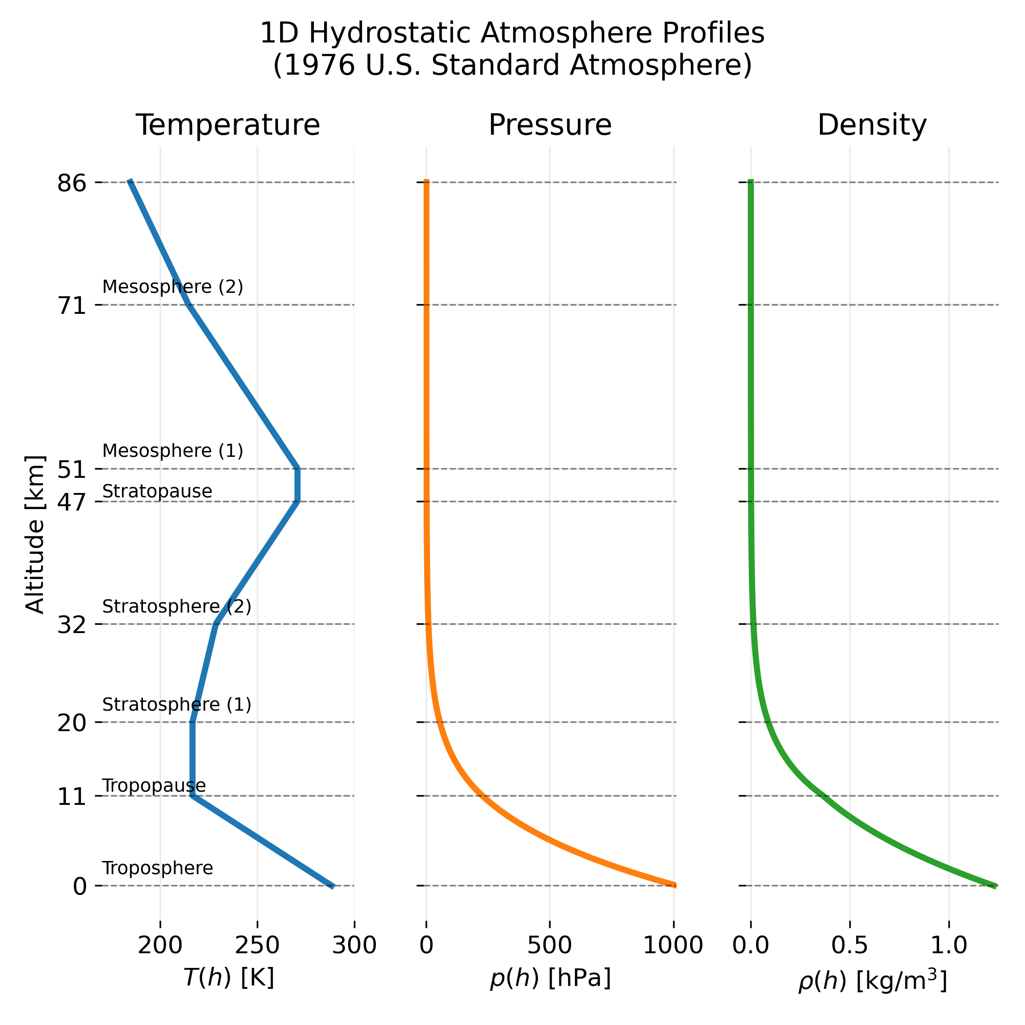
One dimensional hydrostatic atmosphere profiles based on the 1976 U.S. Standard Atmosphere. The left panel shows the prescribed temperature profile, which defines the major atmospheric layers: troposphere, stratosphere, and mesosphere, separated by the tropopause and stratopause. The middle panel shows the corresponding pressure profile obtained from hydrostatic equilibrium, illustrating the rapid decrease of pressure with altitude. The right panel shows the density profile, highlighting the strong vertical stratification of atmospheric mass. All profiles represent a static, horizontally homogeneous reference atmosphere.

Temperature structure and atmospheric layers

The temperature profile defines the classical layering of the atmosphere. Starting at the surface, temperature decreases approximately linearly with altitude in the troposphere (0–11 km). This region is characterized by vigorous vertical mixing and convection, which maintain a nearly constant lapse rate. Weather phenomena are confined almost entirely to this layer.

At about 11 km, the tropopause marks a transition to the stratosphere. In the lower stratosphere (11–20 km), temperature is approximately constant with height, while in the upper stratosphere (20–47 km) temperature increases with altitude. This temperature inversion is caused by the absorption of ultraviolet radiation by ozone, which heats the surrounding air. The top of the stratosphere is referred to as the stratopause.

Above the stratopause lies the mesosphere (47–86 km in this representation), where temperature again decreases with altitude. Radiative cooling dominates in this region, leading to progressively lower temperatures toward the mesopause. The mesosphere is dynamically distinct from the lower atmosphere and plays an important role in wave propagation and energy dissipation.

The piecewise linear temperature structure shown in the plot is not an empirical fit to a single measurement but a standardized approximation that reproduces the mean thermal stratification of the atmosphere.

Pressure profile

The pressure profile decreases monotonically and approximately exponentially with altitude. This behavior is a direct consequence of hydrostatic equilibrium: pressure at a given height reflects the weight of the air column above. Near the surface, pressure decreases rapidly with altitude, while at higher altitudes the gradient becomes much weaker due to the reduced air density.

The pressure profile is largely insensitive to the detailed temperature structure when viewed qualitatively, but quantitative differences between layers arise through the temperature dependence in the hydrostatic equation. The curvature changes across atmospheric layers reflect these temperature variations.

Density profile

The density profile closely mirrors the pressure profile but falls off even more rapidly with altitude. Because density depends on both pressure and temperature, it decreases sharply in the lower atmosphere and becomes extremely small above the stratosphere. By the time the mesosphere is reached, the atmosphere contains only a tiny fraction of the total atmospheric mass.

From a fluid dynamical perspective, this strong vertical density stratification is one of the defining features of the atmosphere. It controls buoyancy, wave propagation, and stability, and it strongly constrains vertical motions.

Numerical ocean profile

For the ocean, idealized but physically plausible temperature and salinity profiles are prescribed. These represent a well mixed surface layer, a thermocline, and the deep ocean.

The hydrostatic equation is solved iteratively because density depends on pressure through the seawater equation of state. At each iteration step, density is evaluated using TEOS 10, and pressure is updated by numerical integration. The resulting profiles are consistent with typical oceanographic reference values and illustrate the strong contrast between the weak compressibility of seawater and the strong pressure increase with depth.

Let’s again start by importing necessary libraries and setting up plotting parameters:

import os
import numpy as np
import matplotlib.pyplot as plt

# TEOS-10 (gsw):
import gsw

# remove spines right and top for better aesthetics:
plt.rcParams['axes.spines.right'] = False
plt.rcParams['axes.spines.top'] = False
plt.rcParams['axes.spines.left'] = False
plt.rcParams['axes.spines.bottom'] = False
plt.rcParams.update({'font.size': 12})

We define physical constants and create an output directory for the figures:

# constants:
g0 = 9.80665          # m/s^2
p_ref = 101325.0      # Pa, reference pressure (not crucial here)
PA_PER_DBAR = 1e4     # 1 dbar = 10^4 Pa (definition)

# output folder:
RESULTS_PATH = "hydrostatic_ocean_1D_figures"
os.makedirs(RESULTS_PATH, exist_ok=True)

Our first function constructs idealized temperature and salinity profiles as functions of depth. Smooth transitions are used to mimic realistic ocean structure:

# idealized ocean profiles:
def idealized_temperature_Salinity(z_m: np.ndarray) -> tuple[np.ndarray, np.ndarray]:
    """
    Construct an idealized T(z) and S(z) profile.

    We use smooth transitions via tanh to mimic:
      * a mixed layer (nearly uniform T, S near surface)
      * a thermocline and halocline
      * deep ocean values

    Parameters
    ----------
    z_m : np.ndarray
        Depth in meters (positive down).

    Returns
    -------
    T_C : np.ndarray
        In situ temperature in degC.
    SP : np.ndarray
        Practical salinity in psu.
    """
    z = np.asarray(z_m, dtype=float)

    # mixed layer thickness and thermocline center and thickness:
    z_ml = 80.0          # m
    z_tc = 600.0         # m
    w_tc = 250.0         # m, transition width

    # surface and deep temperatures:
    T_surface = 20.0     # degC
    T_deep = 2.0         # degC

    # build a smooth decay from surface to deep:
    # f(z) transitions from ~0 near surface to ~1 in deep ocean
    fT = 0.5 * (1.0 + np.tanh((z - z_tc) / w_tc))
    T_C = T_surface * (1.0 - fT) + T_deep * fT

    # enforce a well mixed near surface: flatten T above z_ml;
    # use another smooth switch so there is no sharp kink:
    fML = 0.5 * (1.0 + np.tanh((z - z_ml) / 20.0))
    T_C = (1.0 - fML) * T_surface + fML * T_C

    # salinity: mild surface value, slightly higher at depth, with gentle structure:
    S_surface = 34.6
    S_deep = 34.9
    fS = 0.5 * (1.0 + np.tanh((z - 300.0) / 200.0))
    SP = S_surface * (1.0 - fS) + S_deep * fS

    # add a subtle mid depth maximum (e.g., to mimic an intermediate water mass):
    SP += 0.05 * np.exp(-0.5 * ((z - 1000.0) / 400.0) ** 2)

    return T_C, SP

Next, we define the TEOS-10 based density calculation using the gsw library. This function converts practical salinity and in situ temperature to absolute salinity and conservative temperature before computing density:

# density models:
def rho_teos10(SP: np.ndarray, T_C: np.ndarray, p_dbar: np.ndarray,
               lat: float = 30.0, lon: float = -40.0) -> np.ndarray:
    """
    Compute in situ density using TEOS-10 via gsw.

    We need an approximate location to convert SP, T, p to Absolute Salinity and Conservative Temperature.
    This reference location is a convention. It affects SA conversion slightly.
    For an idealized column, this is acceptable.

    Parameters
    ----------
    SP : np.ndarray
        Practical salinity [psu].
    T_C : np.ndarray
        In situ temperature [degC].
    p_dbar : np.ndarray
        Sea pressure [dbar] (approximately equals absolute pressure minus 1 atm, but gsw expects sea pressure).
    lat, lon : float
        Reference location for SP -> SA conversion.

    Returns
    -------
    rho : np.ndarray
        In situ density [kg/m^3].
    """
    if gsw is None:
        raise RuntimeError("gsw is not available")

    SP = np.asarray(SP, dtype=float)
    T_C = np.asarray(T_C, dtype=float)
    p_dbar = np.asarray(p_dbar, dtype=float)

    SA = gsw.SA_from_SP(SP, p_dbar, lon, lat)     # g/kg
    CT = gsw.CT_from_t(SA, T_C, p_dbar)           # degC
    rho = gsw.rho(SA, CT, p_dbar)                 # kg/m^3
    return rho

Then, we implement the hydrostatic integration function. This function uses fixed point iteration to solve for pressure and density profiles given temperature and salinity profiles. It integrates the hydrostatic equation numerically using the trapezoidal rule:

# hydrostatic integration:
def hydrostatic_ocean_column(
    z_m: np.ndarray,
    T_C: np.ndarray,
    SP: np.ndarray,
    max_iter: int = 30,
    tol_rel: float = 1e-7) -> tuple[np.ndarray, np.ndarray, np.ndarray]:
    """
    Compute hydrostatic pressure and density for a 1D ocean column.

    We solve dp/dz = rho g with rho depending on p via equation of state.
    A fixed point iteration is used because p appears inside rho(S, T, p).

    Parameters
    ----------
    z_m : np.ndarray
        Depth grid [m], increasing from 0.
    T_C : np.ndarray
        Temperature profile [degC].
    SP : np.ndarray
        Salinity profile [psu].
    max_iter : int
        Maximum number of fixed point iterations.
    tol_rel : float
        Relative tolerance on pressure for convergence.

    Returns
    -------
    p_dbar : np.ndarray
        Pressure [dbar].
    rho : np.ndarray
        Density [kg/m^3].
    p_Pa : np.ndarray
        Pressure [Pa].
    """
    z = np.asarray(z_m, dtype=float)
    if np.any(z < 0):
        raise ValueError("Depth z must be >= 0 m.")
    if np.any(np.diff(z) <= 0):
        raise ValueError("Depth grid must be strictly increasing.")

    T_C = np.asarray(T_C, dtype=float)
    SP = np.asarray(SP, dtype=float)
    if T_C.shape != z.shape or SP.shape != z.shape:
        raise ValueError("z, T_C, and SP must have the same shape.")

    # initial pressure guess: assume constant density 1025 kg/m^3:
    rho_guess = 1025.0
    p_Pa = rho_guess * g0 * z
    p_old = p_Pa.copy()

    for _ in range(max_iter):
        p_dbar = p_Pa / PA_PER_DBAR

        rho = rho_teos10(SP, T_C, p_dbar)

        # integrate dp/dz = rho g with trapezoidal rule:
        dp_dz = rho * g0
        p_new = np.zeros_like(z)
        p_new[1:] = np.cumsum(0.5 * (dp_dz[1:] + dp_dz[:-1]) * np.diff(z))

        # convergence check:
        denom = np.maximum(np.abs(p_new), 1.0)
        rel = np.max(np.abs(p_new - p_old) / denom)
        p_Pa = p_new
        if rel < tol_rel:
            break
        p_old = p_Pa.copy()

    # final rho on converged pressure:
    p_dbar = p_Pa / PA_PER_DBAR
    rho = rho_teos10(SP, T_C, p_dbar)

    return p_dbar, rho, p_Pa

After defining the functions, we set up a depth grid, compute the idealized temperature and salinity profiles, and solve for the hydrostatic pressure and density profiles:

# depth grid:
z_max = 5000.0
z_m = np.linspace(0.0, z_max, 900)

# idealized T and S:
T_C, SP = idealized_temperature_Salinity(z_m)

# hydrostatic column:
p_dbar, rho, _p_Pa = hydrostatic_ocean_column(z_m, T_C, SP)

# some plot settings:
z_km = z_m * 1e-3 # convert to km

# depth ticks (km):
depth_ticks_km = np.array([0, 0.1, 0.5, 1, 2, 3, 4, 5], dtype=float)


# plotting:
fig, axs = plt.subplots(1, 4, figsize=(7, 7), sharey=True)

# plot temperature:
axs[0].plot(T_C, z_km, lw=3, c="tab:blue")
axs[0].set_xlabel(r"$T(z)$ [°C]")
axs[0].set_ylabel("Depth [km]")
axs[0].set_title("Temperature")
axs[0].set_ylim(depth_ticks_km[-1], depth_ticks_km[0])

# plot pressure:
axs[1].plot(p_dbar, z_km, lw=3, c="tab:orange")
axs[1].set_xlabel(r"$p(z)$ [dbar]")
axs[1].set_title("Pressure")

# plot density:
axs[2].plot(rho, z_km, lw=3, c="tab:green")
axs[2].set_xlabel(r"$\rho(z)$ [kg/m$^3$]")
axs[2].set_title("Density")

# plot salinity:
axs[3].plot(SP, z_km, lw=3, c="tab:purple")
axs[3].set_xlabel(r"$S(z)$ [psu]")
axs[3].set_title("Salinity")
# optional, but typically nice for readability:
axs[3].set_xlim(np.min(SP) - 0.1, np.max(SP) + 0.1)

# annotate typical layers on the left panel:
axs[0].text(np.min(T_C), 0.15, "Mixed layer", fontsize=10, va="center")
axs[0].text(np.max(T_C), 0.8, "Thermocline", fontsize=10, va="center", ha="right")
axs[0].text(np.max(T_C), 3.0, "Deep ocean", fontsize=10, va="center", ha="right")

# depth axis direction: ocean increases downward, so invert y-axis:
for ax in axs:
    ax.set_yticks(depth_ticks_km)
    ax.grid(True, alpha=0.25)
    ax.invert_yaxis()

# title:
thermo_label = "TEOS-10 (gsw)"
fig.suptitle(f"1D Hydrostatic Ocean Column Profiles\n(idealized T and S, {thermo_label})", fontsize=14)

fig.tight_layout()

outpath = os.path.join(RESULTS_PATH, "hydrostatic_ocean_1D_profiles.png")
plt.savefig(outpath, dpi=300)
plt.close(fig)

Also for this example, a full version of the script is available in the GitHub repository mentioned at the end of this post.

Discussion of the ocean profiles

The generated plot shows idealized one dimensional vertical profiles of temperature, pressure, density, and salinity for a static ocean column in hydrostatic equilibrium. In contrast to the atmospheric case, the vertical coordinate is depth, measured positively downward from the sea surface. The profiles are computed using prescribed temperature and salinity structures and a thermodynamically consistent equation of state for seawater (TEOS-10).

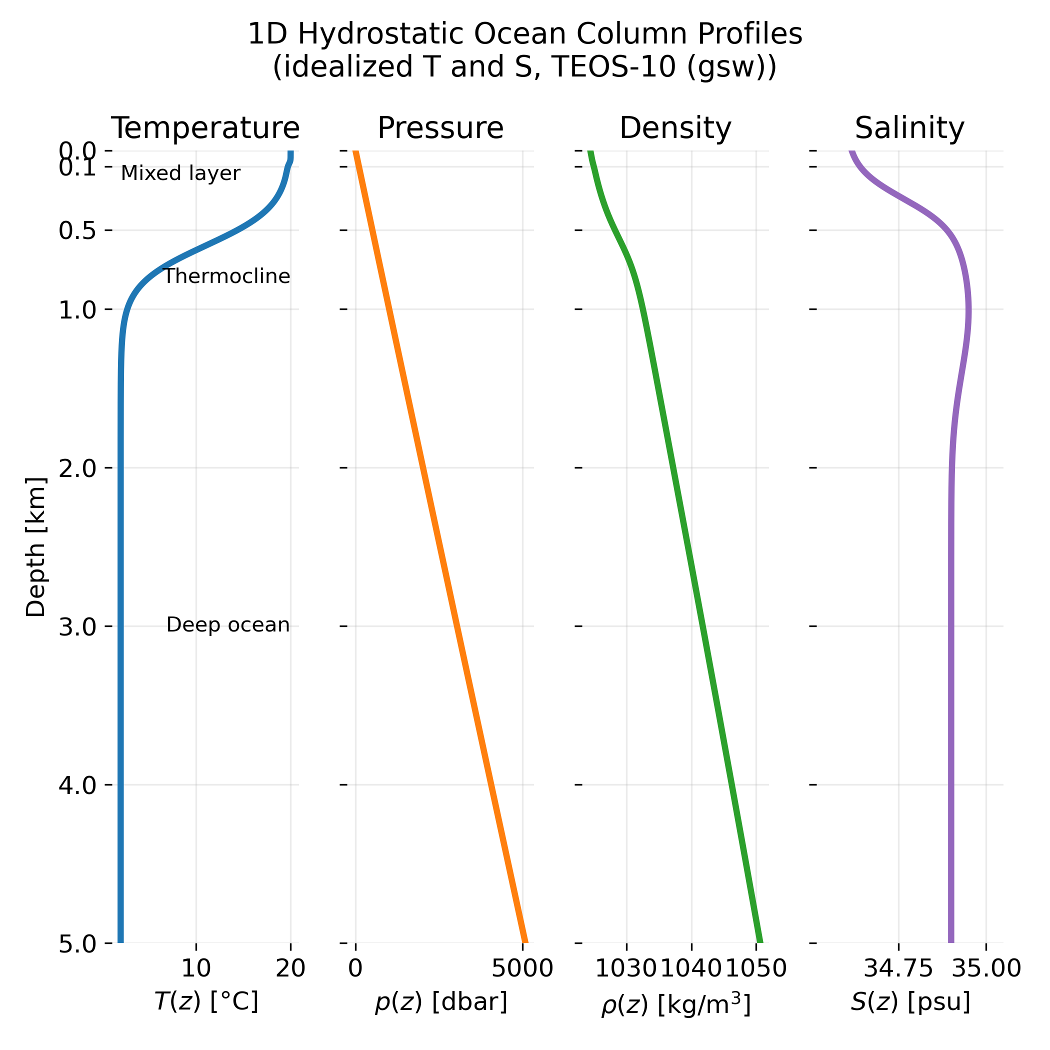
One dimensional hydrostatic ocean column profiles computed from idealized temperature and salinity distributions using the TEOS-10 seawater equation of state. The left panel shows the temperature profile, defining the mixed layer, thermocline, and deep ocean. The second panel shows the hydrostatic pressure profile, which increases approximately linearly with depth due to the weak compressibility of seawater. The third panel shows the corresponding in situ density profile, highlighting the stable stratification of the ocean interior. The right panel shows the salinity profile, illustrating relatively small but dynamically important vertical variations. All profiles represent a static, horizontally homogeneous reference ocean column.

Although strongly simplified, the profiles capture the essential vertical organization of the ocean and illustrate the physical mechanisms that distinguish oceanic stratification from that of the atmosphere.

Temperature structure and oceanic layers

The temperature profile defines the major vertical layers of the ocean. Near the surface, the mixed layer is characterized by nearly uniform temperature. This layer is maintained by wind driven turbulence, surface cooling, and wave induced mixing, which efficiently homogenize temperature over tens of meters to a few hundred meters, depending on location and season.

Below the mixed layer lies the thermocline, a transition region in which temperature decreases rapidly with depth. This strong vertical gradient reflects the limited penetration of surface heating and the suppression of vertical mixing by stable stratification. The thermocline acts as a dynamical barrier that separates surface processes from the deep ocean.

At greater depths, the deep ocean is characterized by weak vertical temperature gradients and low temperatures that vary only slowly with depth. These water masses are typically formed at high latitudes and fill the ocean interior through large scale circulation.

The smooth temperature transitions shown in the plot are idealized representations of these processes rather than direct observations.

Pressure profile

The pressure profile increases almost linearly with depth. This reflects the near incompressibility of seawater: because density varies only weakly with pressure and depth, the hydrostatic relation implies an approximately linear pressure increase.

In oceanography, pressure is commonly expressed in decibar. A useful rule of thumb is that pressure increases by roughly one decibar per meter of depth, which is evident in the plotted profile. Unlike in the atmosphere, where pressure decreases exponentially with height, the oceanic pressure profile is simple and monotonic.

Density profile

The density profile shows a gradual increase with depth. This increase results from two contributions: cooling with depth, which increases density through thermal contraction, and the direct compressive effect of pressure on seawater.

Compared to the atmosphere, density variations in the ocean are small in relative terms, typically only a few percent over the full water column. Nevertheless, these small variations are dynamically crucial. Even weak density gradients are sufficient to strongly inhibit vertical motion and mixing, making density stratification a central organizing principle of ocean dynamics.

The slight curvature of the density profile reflects the combined influence of temperature, salinity, and pressure through the nonlinear seawater equation of state.

Salinity structure

The salinity profile exhibits comparatively weak vertical variations. Near the surface, salinity can be influenced by evaporation, precipitation, river input, and ice processes, leading to modest deviations from the deep ocean value.

At greater depths, salinity becomes nearly uniform, reflecting the long time scales over which deep ocean water masses are formed and mixed. The subtle salinity structure shown here illustrates that, although salinity variations are small, they contribute significantly to density and therefore to stratification and circulation.

Conclusion

The hydrostatic atmosphere and ocean profiles presented here illustrate how much of the large scale vertical structure of both systems can be understood from a small set of fundamental fluid dynamical principles. In both cases, the dominant balance is between pressure gradients and gravity, and the resulting hydrostatic equilibrium provides a natural reference state around which more complex dynamics unfold.

For the atmosphere, the combination of hydrostatic balance with the ideal gas law leads to analytically tractable solutions once a temperature profile is prescribed. The resulting pressure and density profiles reveal the strong compressibility of air and the exponential decrease of mass with altitude. The temperature structure, in turn, defines the classical atmospheric layers and reflects the interplay between radiative processes and vertical stability.

In the ocean, the same hydrostatic principle applies, but the physics is shaped by a fundamentally different equation of state. Weak compressibility, combined with a strong dependence of density on temperature and salinity, produces a vertical structure in which pressure increases almost linearly with depth while density varies only slightly. Despite their small magnitude, these density variations control stratification, suppress vertical motion, and govern the coupling between surface forcing and the deep ocean.

I did not put the atmosphere and the ocean into a single post without a certain intention. I think, placing both side by side highlights both their unity and their contrast. Both are fluids under gravity governed by the same mechanical balance, yet their thermodynamic properties lead to qualitatively different vertical structures and dynamical behavior. The simple one dimensional models discussed here do not aim to describe real weather or circulation, but they provide physically transparent baseline states. Such reference profiles are indispensable for understanding buoyancy, stability, wave propagation, and for interpreting more complex numerical models of the coupled Earth system.

Update and code availability: This post and its accompanying Python code were originally drafted in 2021 and archived during the migration of this website to Jekyll and Markdown. In January 2026, I substantially revised and extended the code. The updated and cleaned-up implementation is now available in this new GitHub repositoryꜛ. Please feel free to experiment with it and to share any feedback or suggestions for further improvements.

References and further reading

• Mallat, S.A Wavelet Tour of Signal Processing, 2008, Academic Press. ISBN: 978-0123743701
• Daubechies, I., Ten Lectures on Wavelets, 1992 SIAM. ISBN: 978-0898712742
• Kaiser, G., A Friendly Guide to Wavelets, 1994, Birkhäuser. ISBN: 978-0817637914
• Oppenheim, A. V. & Schafer, R. W., Discrete-Time Signal Processing, 2009 Pearson. ISBN: 978-0131988422
• Hans-Georg Stark, Wavelets and Signal Processing: An Application-Based Introduction, 2005, Springer Berlin Heidelberg, ISBN: 3-540-23433-0
• Alfred Karl Louis, Peter Maaß, and Andreas Rieder, Wavelets, Theorie und Anwendungen, 1998, Teubner, ISBN: 13:978-3-519-12094-0
• Silvia Bacchelli, Serena Papi, 2006, Image denoising using principal component analysis in the wavelet domain, Journal of Computational and Applied Mathematic, Volume 189, Issues 1–2, Pages 606-621, ISSN 0377-0427, DOI: 10.1016/j.cam.2005.04.030ꜛ
• Walter Greiner, Horst Stock, Hydrodynamik - Ein Lehr- und Übungsbuch; mit Beispielen und Aufgaben mit ausführlichen Lösungen, 1991, Harri Deutsch Verlag, ISBN: 9783817112043
• Heinz Schade and Ewald Kunz, Strömungslehre, 2007, de Gruyter, ISBN: 978-3-11-018972-8
• Sirovich Antman, J. E. Marsden, Hale P Holmes, J. Keller, J. Keener, B. J. Mielke, A. Matkowsky, C. S. Sreenivasan, and K. R. S. Perkin, Prandtl’s Essential of Fluid Mechanics, 2004, Vol. 158, Springer, ISBN: 0-387-40437-6
• O. G. Drazin, Introduction to hydrodynamic stability, 2002, Cambridge University Press, ISBN: 0521 80427 2
• Rutherford Aris, Vectors, tensors and the basic equations of fluid mechanics, 1962, Dover Publications Inc., ISBN: 0-486-66110-5
• Jianping Zhu, Computational Simulations and Applications, 2011, Intechweb.org, ISBN: 978-953-307-430-6
• Pieter Wesseling, Principles of computational fluid dynamics, 2001, Springer-Verlag, ISBN: 3-540-67853-0
• Franz Durst, Grundlagen der Strömungslehre, 2006, Springer-Verlag, ISBN: 978-3-540-31323-6
• Wilhelm Kley, Numerische Hydrodynamik, 2004, Universitaet Tuebingen (Lecture Notes)
• Burg, K., Haf, H., Wille, F., & Meister, A. Partielle Differentialgleichungen und funktionalanalytische Grundlagen, 2010, 5th ed., Vieweg + Teubner, ISBN: 978-3-8348-1294-0
• Lord Kelvin (William Thomson), Hydrokinetic solutions and observations, 1871, Philosophical Magazine. 42: 362–377
• Hermann von Helmholtz, Über discontinuierliche Flüssigkeits-Bewegungen [On the discontinuous movements of fluids]”, 1868, Monatsberichte der Königlichen Preussische Akademie der Wissenschaften zu Berlin. 23: 215–228
• Lewis Fry Richardson, Weather Prediction by Numerical Process, 1922, Cambridge University Press, ISBN: 9780521680448, archive.orgꜛ
• Kolmogorov, A. N., The local structure of turbulence in incompressible viscous fluid for very large Reynolds numbers, 1890, Vol. 434, No. 1890, Turbulence and Stochastic Process: Kolmogorov’s Ideas 50 Years On (Jul. 8, 1991), pp. 9-13, online PDFꜛ
• Frisch, U., Turbulence: the legacy of A. N. Kolmogorov, 1995/2010, Cambridge University Press, ISBN: 978-0521457132
• Pope, S. B., Turbulent flows, 2000, Cambridge University Press, ISBN: 978-0521598866
• Davidson, P. A., Turbulence: an introduction for scientists and engineers, 2015, Oxford University Press, ISBN: 978-0198722595