Understanding Hebbian learning in Hopfield networks
Hopfield networks, a form of recurrent neural network (RNN), serve as a fundamental model for understanding associative memory and pattern recognition in computational neuroscience. Central to the operation of Hopfield networks is the Hebbian learning rule, an idea encapsulated by the maxim “neurons that fire together, wire together”. In this post, we explore the mathematical underpinnings of Hebbian learning within Hopfield networks, emphasizing its role in pattern recognition.
Hopfield networks
A Hopfield network consists of a set of neurons that are either in an “on” (+1) or “off” (-1) state (these class of neurons is also called binary McCulloch-Pitts neurons). The network belongs to the class of feedback networks and consists of only one layer, which simultaneously functions as an input and output layer. The network is fully connected, i.e., each neuron is connected to every other neuron with a certain weight, except to itself. These weights determine the network’s dynamics and are adjusted according to the Hebbian learning rule to store specific patterns.
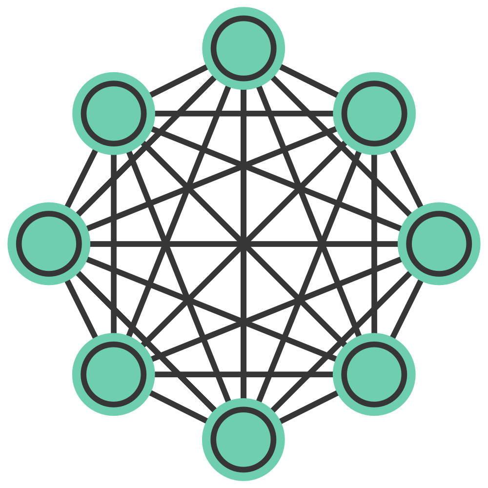 Diagram of a Hopfield network. All neurons are connected to each other with a certain weight, except to itself. The so-called McCulloch-Pitts neurons can have a state of +1 or -1.
Mathematical foundation
The weight $w_{ij}$ between two neurons $i$ and $j$ in a Hopfield network is updated based on the Hebbian learning principle as follows:
\[w_{ij} = \frac{1}{N} \sum_{\mu=1}^P \xi_i^\mu \xi_j^\mu\]where:
- $N$ is the total number of neurons in the network,
- $P$ is the number of patterns to be memorized,
- $\xi_i^\mu$ is the state (-1 or 1) of neuron $i$ in pattern $\mu$.
Diagonal elements of the weight matrix are set to zero, $w_{ii} = 0$ to prevent neurons from influencing themselves (as no self-connections are allowed). In a binary pattern consisting of just 1s and -1s, $\xi_i^\mu$ corresponds to the value of the $i$-th element of the $\mu$-th pattern. Thus, we can set $\xi_i^\mu = 1$ if the $i$-th element of the $\mu$-th pattern is 1, and $\xi_i^\mu = -1$ if the $i$-th element of the $\mu$-th pattern is -1, i.e., $\xi^\mu = \text{pattern}^\mu$.
The above formula ensures that the weights are adjusted to reinforce the correlation between neurons that are simultaneously active across the stored patterns. The training process involves adjusting the weights based on the provided patterns. This operation effectively implements the Hebbian learning rule, reinforcing the connection between neurons that are concurrently on in the same pattern.
Once trained, the Hopfield network can recognize patterns by evolving from a given initial state (which can be a noisy or incomplete version of a stored pattern) towards a stable state that corresponds to one of the memorized patterns. This process is mathematically represented as:
\[s_i^{(t+1)} = \text{sgn}\left(\sum_{j} w_{ij} s_j^{(t)}\right)\]where $s_i^{(t+1)}$ is the state of neuron $i$ at time $t+1$, and $\text{sgn}(\cdot)$ is the sign function, which ensures the neuron state is updated to either +1 or -1 based on the weighted sum of its inputs.
Application to pattern recognition
To demonstrate the application of Hebbian learning in pattern recognition using Hopfield networks, let’s start by implementing a simple Hopfield network class in Python:
class HopfieldNetwork:
    def __init__(self, size):
        self.size = size
        self.weights = np.zeros((size, size))
Next, we add a method to train the network using the Hebbian learning rule:
    def train(self, patterns):
        for pattern in patterns:
            pattern = np.reshape(pattern, (self.size, 1)) # reshape to a column vector
            self.weights += np.dot(pattern, pattern.T) # update weights based on Hebbian learning rule, i.e., weights = weights + pattern*pattern'
        self.weights[np.diag_indices(self.size)] = 0 # set diagonal to 0 in order to avoid self-connections
        self.weights /= self.size # normalize weights by the number of neurons to ensure stability of th network
In this training function, we iterate over the provided patterns and update the weights based on the Hebbian learning rule. We then normalize the weights by the number of neurons to ensure the stability of the network.
Finally, we add a method to predict the network’s output based on a given input:
    def predict(self, pattern, steps=10):
        pattern = pattern.copy()
        for _ in range(steps):
            for i in range(self.size):
                raw_value = np.dot(self.weights[i, :], pattern)
                pattern[i] = 1 if raw_value >= 0 else -1
        return pattern
The prediction function illustrates how a Hopfield network can recover stored patterns from corrupted inputs. It updates each neuron’s state based on the current pattern and the learned weights, iteratively moving the network towards a stable state that corresponds to one of the memorized patterns.
That’s almost everything we need to implement a simple Hopfield network in Python. We can now use this class to train the network on a set of patterns and then test its ability to recover these patterns from noisy or incomplete inputs. Below is the complete Python code for the Hopfield network class and an example of its usage:
import numpy as np
import matplotlib.pyplot as plt

# define the Hopfield network class:
class HopfieldNetwork:
    def __init__(self, size):
        self.size = size
        self.weights = np.zeros((size, size))

    def train(self, patterns):
        for pattern in patterns:
            pattern = np.reshape(pattern, (self.size, 1)) # reshape to a column vector
            self.weights += np.dot(pattern, pattern.T) # update weights based on Hebbian learning rule, i.e., W = W + p*p'
        self.weights[np.diag_indices(self.size)] = 0 # set diagonal to 0 in order to avoid self-connections
        self.weights /= self.size # normalize weights by the number of neurons to ensure stability of th network

    def predict(self, pattern, steps=10):
        pattern = pattern.copy()
        for _ in range(steps):
            for i in range(self.size):
                raw_value = np.dot(self.weights[i, :], pattern)
                pattern[i] = 1 if raw_value >= 0 else -1
        return pattern

    def visualize_patterns(self, patterns, title):
        fig, ax = plt.subplots(1, len(patterns), figsize=(10, 5))
        for i, pattern in enumerate(patterns):
            ax[i].matshow(pattern.reshape((int(np.sqrt(self.size)), -1)), cmap='binary')
            ax[i].set_xticks([])
            ax[i].set_yticks([])
        fig.suptitle(title)
        plt.show()

# define test patterns
pattern1 = np.array([-1,1,1,1,1,-1,-1,1,-1]) # representing a simple shape
pattern2 = np.array([1,1,1,-1,1,1,-1,-1,-1]) # another simple shape
patterns = [pattern1, pattern2]

# initialize Hopfield network:
network_size = 9 # this should be square to easily visualize patterns
hn = HopfieldNetwork(network_size)

# train the network:
hn.train(patterns)

# corrupt patterns slightly:
corrupted_pattern1 = np.array([-1,1,-1,1,1,-1,-1,1,-1]) # slightly modified version of pattern1
corrupted_pattern2 = np.array([1,1,1,-1,-1,1,-1,-1,-1]) # slightly modified version of pattern2
corrupted_patterns = [corrupted_pattern1, corrupted_pattern2]

# predict (recover) from corrupted patterns:
recovered_patterns = [hn.predict(p) for p in corrupted_patterns]

# visualize original, corrupted, and recovered patterns:
hn.visualize_patterns(patterns, 'Original Patterns')
hn.visualize_patterns(corrupted_patterns, 'Corrupted Patterns')
hn.visualize_patterns(recovered_patterns, 'Recovered Patterns')
Note, that I added an additional visualize_patterns method to the HopfieldNetwork class to visualize the patterns. We define two patterns,
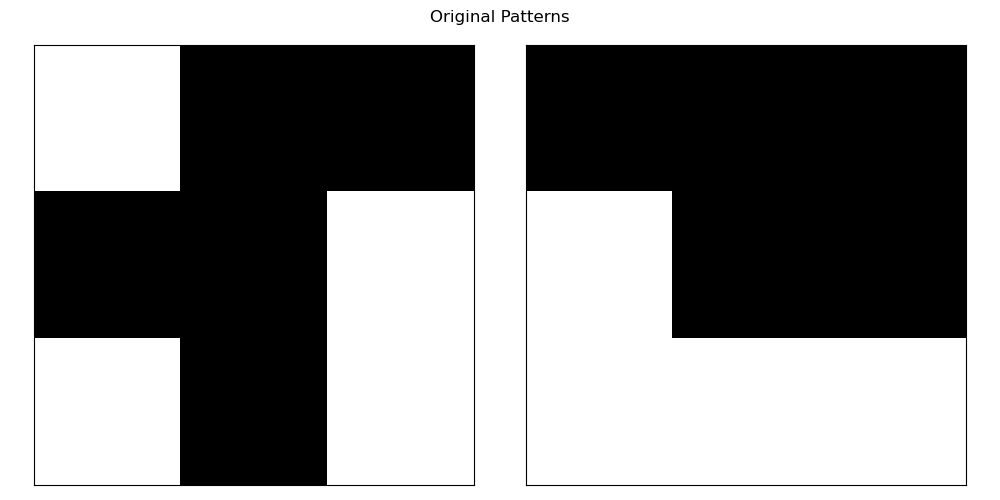
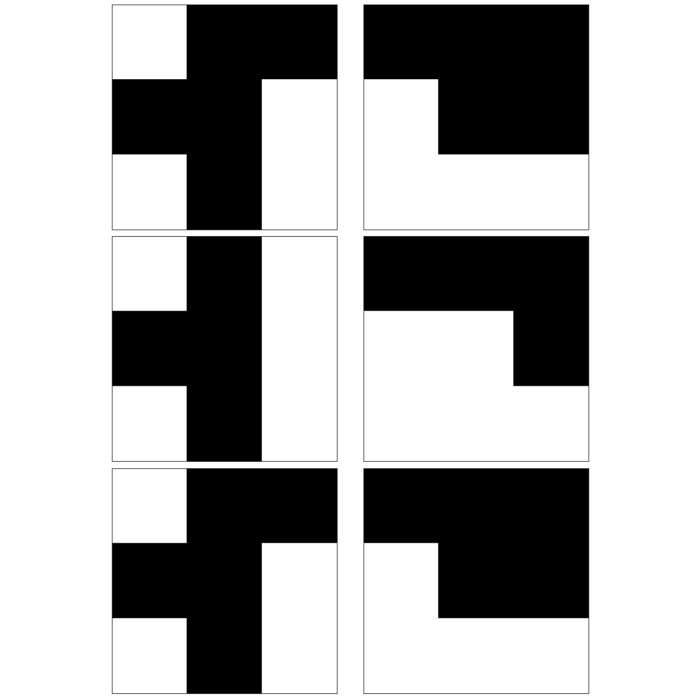
and train the network on these patterns. We then slightly corrupt the patterns,
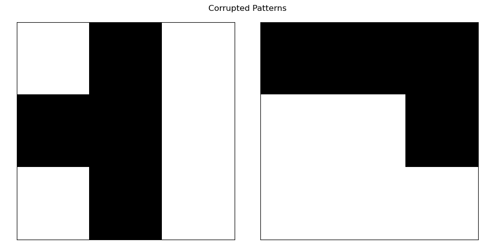
and use the trained network to recover the original patterns from the corrupted versions:

From the recovered patterns, we can see that the Hopfield network successfully recovered the original patterns from the corrupted versions, demonstrating that the network has learned to recognize and recall the memorized patterns.
Conclusion
Hebbian learning forms the core of Hopfield networks, enabling them to store and recognize patterns. Through iterative adjustments of neuronal connections based on the principle that “neurons that fire together, wire together”, Hopfield networks can recover original patterns from noisy or incomplete versions, showcasing their utility in pattern recognition tasks. The mathematical formulation and Python implementation presented here hopefully offer a foundational understanding of how Hopfield networks operate. You can play around with the code to train the network on different patterns and observe its ability to recover them from corrupted inputs. Adding noise to the patterns and testing the network’s robustness is also an interesting experiment to try.
You can find the complete code for this post also in this GitHub repositoryꜛ.
References
- Hopfield, John J., Neural networks and physical systems with emergent collective computational abilities, 1982, Proc Natl Acad Sci U S A, 79(8), 2554-2558. doi: 10.1073/pnas.79.8.2554
- Hopfield, John J., Neurons with graded response have collective computational properties like those of two-state neurons, 1984, Proc Natl Acad Sci U S A, 81(10), 3088-3092. doi: 10.1073/pnas.81.10.3088
- Hebb, Donald O. , The Organization of Behavior, 1949, Wiley: New York, pages 437, url, doi: 10.1016/s0361-9230(99)00182-3
- Wulfram Gerstner, Werner M. Kistler, Richard Naud, and Liam Paninski, Neuronal Dynamics: From Single Neurons to Networks and Models of Cognition, 2014, Cambridge University Press, https://www.cambridge.org/9781107060838, Online-Version
Comments
Comment on this post by publicly replying to this Mastodon post using a Mastodon or other ActivityPub/Fediverse account.
Comments on this website are based on a Mastodon-powered comment system. Learn more about it here.
There are no known comments, yet. Be the first to write a reply.