Using phase plane analysis to understand dynamical systems

When it comes to understanding the behavior of dynamical systems, analyzing the system’s behavior directly from its differential equations can often be too complex. In such situations, phase plane analysis can be a powerful tool for gaining insights into the system’s dynamics. By plotting the system’s state variables against each other, this method provides a clear and intuitive representation of the system’s behavior, making it easier to visualize and interpret complex dynamical phenomena. This approach is particularly valuable in computational neuroscience, where systems of differential equations model the behavior of neurons and neural networks. Through phase plane analysis, it’s possible to discern important dynamic properties of these models, such as the occurrence of oscillations represented by limit cycles. These oscillations are fundamental to many neural functions, including rhythm generation and pattern recognition, highlighting the method’s significance in exploring and understanding the underlying mechanisms of neural activity. Here, we explore how we can use phase plane analysis to understand and interpret the behavior of such dynamical systems.

Mathematical foundation

Suppose we have a system of two first-order ordinary differential equations (ODEs) of the form:

\[\begin{align*} \dot{x} &= f(x, y), \\ \dot{y} &= g(x, y), \end{align*}\]

where $x$ and $y$ are the state variables, $\dot{x}$ and $\dot{y}$ are their respective time derivatives, and $f(x, y)$ and $g(x, y)$ are the functions that define the system’s dynamics. The phase plane is a two-dimensional space defined by the state variables $x$ and $y$. Each point $(x, y)$ in this space represents a unique state of the system, and the system’s dynamics can be visualized by plotting the system’s trajectories, $(\dot{x}, \dot{y})$, in this space.

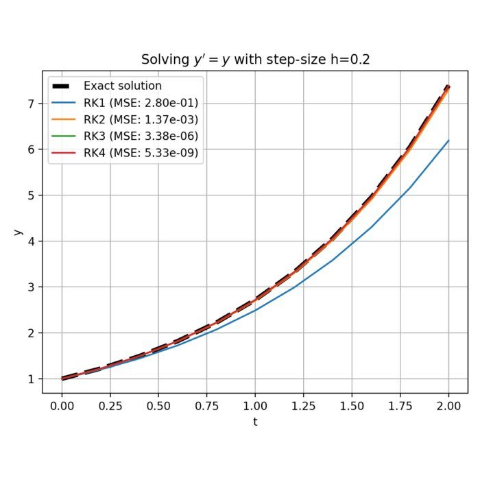
Since it is often not possible to solve the system of ODEs analytically, numerical methods are used to calculate the trajectories of the system in the phase plane. The most common method for this purpose is the Runge-Kutta method, which is a family of implicit and explicit iterative methods, used in temporal discretization for the approximate solutions of ordinary differential equations.

Limit cycles

A limit cycle is a closed trajectory in the phase plane that represents stable, unstable or semi-stable periodic solutions of the system. Graphically, the existence of limit cycles can be determined by the drawn vector fields and trajectories of the system in the phase plane. Limit cycles are identified by finding closed curves that are neither crossed inwards nor outwards by trajectories.

A limit cycle fulfills the condition that a starting point $(x_0, y_0)$ on the cycle is valid after a period $T$:

\[x(T + t_0) = x(t_0) \quad \text{and} \quad y(T + t_0) = y(t_0)\]

for all $t_0$, where $x(t)$ and $y(t)$ are the solutions of the above differential equations.

Nullclines

A useful tool for phase plane analysis are the nullclines. A nullcline is a curve in the phase plane where one of the state variables has a zero derivative,

\[\begin{align*} \dot{x} &= 0 \\ \dot{y} &= 0 \end{align*}\]

i.e., set $f(x, y) = 0$ and $g(x, y) = 0$ to find the x- and y-nullclines, respectively. The nullclines can be used to identify the equilibrium points of the system and to visualize the system’s dynamics. The intersection points of the nullclines are the equilibrium points of the system, where the system’s state variables do not change over time. The nullclines divide the phase plane into regions of different dynamics and help to understand the behavior of the system, in particular the tendency of trajectories to move along or away from these curves. The shape of the nullcline and its position relative to the state variables $x$ and $y$ are crucial for analyzing the stability and the possible existence of limit cycles in the system.

Local behavior and stability analysis

The local stability of a limit cycle can be determined by linearizing the (nonlinear) system along the cycle in the vicinity of equilibrium points and examining the eigenvalues of the resulting Jacobian matrix:

\[J = \begin{bmatrix} \frac{\partial f}{\partial x} & \frac{\partial f}{\partial y} \\ \frac{\partial g}{\partial x} & \frac{\partial g}{\partial y} \end{bmatrix}_{\text{along the limit cycle}}\]

The eigenvalues of the Jacobian matrix provide information about stability. Their signs indicate whether trajectories converge to or diverge from the equilibrium point, defining the state of the limit cycle, which is

• stable if all eigenvalues of $J$ have negative real parts, signifying that the eigenvectors outline stable states towards which the system is drawn, with their intersection forming a stable node,
• unstable if at least one eigenvalue has a positive real part, indicating that the eigenvectors depict unstable states away from which the system tends to move, marking the intersection as an unstable node;
• semi-stable if the eigenvalues have both positive and negative real parts, resulting in a saddle point at the intersection of the eigenvectors; this scenario indicates trajectories near this point are attracted in one direction while being repelled in the perpendicular direction.

The eigenvectors indicate the directions in which this convergence or divergence is strongest and define the main axes along which the dynamics of the system unfold.

It can also be analytically challenging to explicitly calculate the eigenvalues of $J$, especially for higher-dimensional systems. In such cases, numerical methods can be used to calculate the eigenvalues and determine the stability of the limit cycle. Another approach is to graphically identify the stability of the limit cycle by examining the behavior of the system’s trajectories near the cycle.

To interpret the behavior of the system around equilibrium points graphically, straight lines in the phase plane are plotted to represent the eigenvectors associated with the eigenvalues of the Jacobian matrix. To illustrate the eigenvectors and the behavior of the nodes in a dynamic system, we exemplarily use simplified linear systems of differential equations defined by the matrices $A$ in the code below. The eigenvalues and eigenvectors of these matrices determine the behavior of each system near theirs equilibrium points (typically the origin):

import numpy as np
import matplotlib.pyplot as plt
from scipy.linalg import eig
from numpy import real

# define systems:
A_saddle   = np.array([[2, 0], [0, -2]])  # saddle point
A_instable = np.array([[2, 0], [0, 2]])   # unstable node
A_stable   = np.array([[-2, 0], [0, -2]]) # stable knot

# calculate eigenvalues and eigenvectors:
eigvals_saddle, eigvecs_saddle = eig(A_saddle)
eigvals_instable, eigvecs_instable = eig(A_instable)
eigvals_stable, eigvecs_stable = eig(A_stable)

 # plot the phase portraits for each system:
def plot_phase_portrait(A, eigvecs, eigvals, title):
    fig, ax = plt.subplots(figsize=(6, 6))
    x, y = np.meshgrid(np.linspace(-5, 5, 20), np.linspace(-5, 5, 20))
    u = A[0, 0] * x + A[0, 1] * y
    v = A[1, 0] * x + A[1, 1] * y
    ax.streamplot(x, y, u, v, color='b')
    for vec in eigvecs.T:
        ax.quiver(0, 0, 3*real(vec[0]), 3*real(vec[1]), scale=1, 
                  scale_units='xy', angles='xy', color='r')
    ax.set_title(title+f"\neigenvalues (real part): {real(eigvals)}")
    ax.axis('equal')
    plt.tight_layout()
    plt.savefig(f'eigenvectors_and_nodes_{title}.png', dpi=120)
    plt.show()

# saddle point:
plot_phase_portrait(A_saddle, eigvecs_saddle, eigvals_saddle, 'saddle point')

# unstable node:
plot_phase_portrait(A_instable, eigvecs_instable, eigvals_instable, 'unstable node')

# stable knot:
plot_phase_portrait(A_stable, eigvecs_stable, eigvals_stable, 'stable knot')

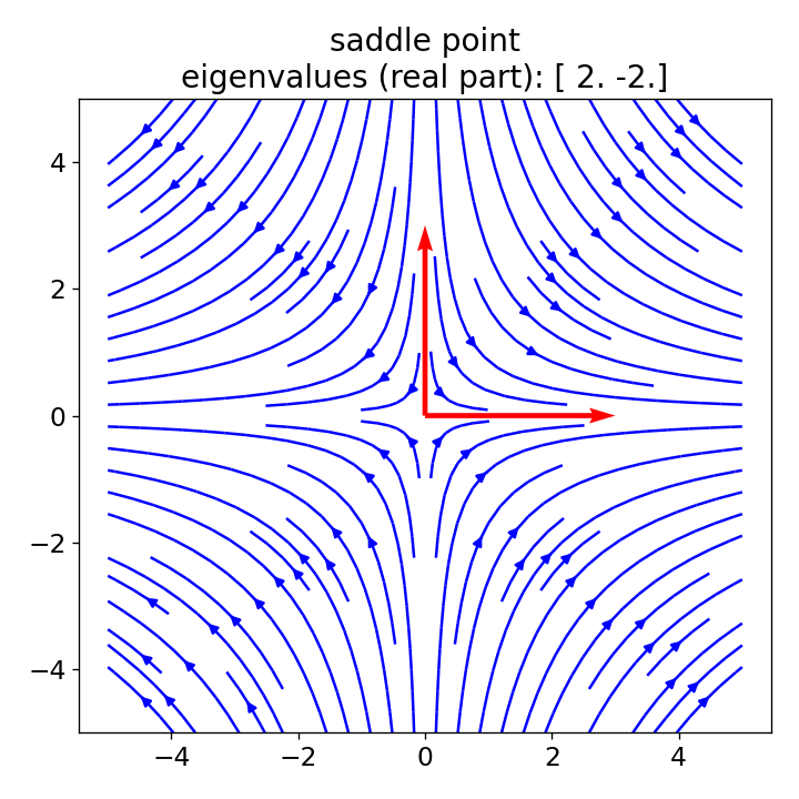
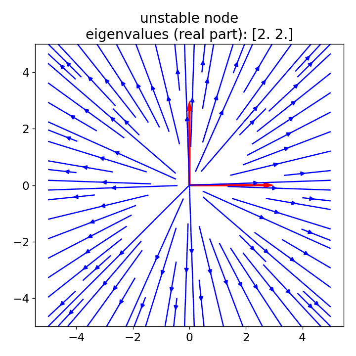
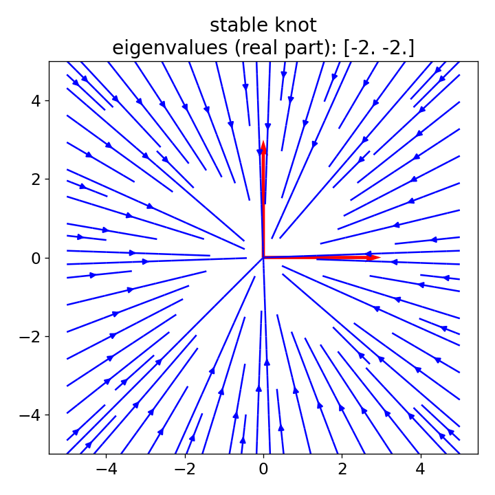Vector fields (blue) for a saddle point (left), unstable node (center), and stable knot (right) scenario. Eigenvectors are depicted in red.

In these plots, red lines represent the eigenvectors, illustrating the main axes of the system dynamics, while the blue lines depict the vector field of the system, i.e., its dynamics. Each plots demonstrates one of the three scenarios described above:

1. saddle point: The system’s trajectories are attracted towards the equilibrium along the eigenvector associated with the negative eigenvalue (stable) and repelled away along the eigenvector associated with the positive eigenvalue (unstable).
2. unstable node: Here, both eigenvalues are positive, indicating that trajectories are repelled from the equilibrium point in the directions aligned with both eigenvectors. The system’s dynamics indicate that any small perturbation will cause the state to move away from the equilibrium, growing fast over time.
3. stable node: In this case, both eigenvalues are negative, meaning trajectories are attracted to the equilibrium point towards the origin of both eigenvectors. The dynamics show that any perturbation will decay, bringing the state back to equilibrium over time.

Note, that the matrices used in this example (A_saddle, A_instable, and A_stable) mimic a very simplified linear system. Each of these matrices is already diagonal (off-diagonal elements are zero). This structural characteristic directly influences the orientation of the eigenvectors, in our case having the eigenvectors aligned with the x- and y-axis (they correspond to the diagonal elements of the chosen matrices; and since there’s no off-diagonal term to create a rotation or a shear, the direction of the eigenvectors naturally aligns with the axes). And the origin of the eigenvectors is at (0,0), which serves as the equilibrium point (or fixed point) for these systems because it is the point where both the rate of change of $x$ and $y$ are zero given the systems’ dynamics.

Example: Simple pendulum

The simple pendulum is a classical example of a dynamical system that can be easily analyzed using phase plane analysis. The system is described by the following ODE:

\[\frac{d^2\theta}{dt^2} + \frac{g}{l}\sin(\theta) = 0\]

with $\theta$ the angle of deflection of the pendulum from the vertical, $g$ the acceleration due to gravity ($9.81 \, \text{m/s}^2$), and $l$ the length of the pendulum rope. We assume that there is no friction or air resistance. The potential energy $U$ of the pendulum is given by

\[U = mgh = mgl(1 - \cos(\theta))\]

where $m$ is the mass of the pendulum bob and $h$ is the height above the lowest position. Without loss of generality, we can set $m = 1$ and $l = 1$ to simplify the calculation.

The phase portrait of a pendulum can be obtained by converting the second order differential equation into a first order system. We introduce a new variable $v = \frac{d\theta}{dt}$ so that we have:

\[\begin{align*} \frac{d\theta}{dt} &= v \\ \frac{dv}{dt} &= -\frac{g}{l}\sin(\theta) \end{align*}\]

The nullclines of the pendulum system are given by the conditions under which the derivatives $\frac{d\theta}{dt}$ and $\frac{dv}{dt}$ are zero. The $v$-nullcline is determined by setting $\frac{d\theta}{dt} = 0$. This condition is met when $v = 0$, which corresponds to the pendulum being at its highest or lowest point in its swing, where it momentarily stops before reversing direction. In the phase plane, this nullcline is represented by a horizontal line at $v = 0$, indicating that there is no change in the angle $\theta$ at these points.

The $\theta$-nullcline is found by setting $\frac{dv}{dt} = 0$, which occurs when $\sin(\theta) = 0$. This condition is satisfied for $\theta = n\pi$, where $n$ is any integer. Physically, these points correspond to the pendulum being in the vertical position, either hanging down or standing up. In the phase portrait, these nullclines are represented by vertical lines at each multiple of $\pi$ for $\theta$, indicating positions of equilibrium where the pendulum’s velocity does not change because the gravitational force is either perfectly balanced or there is no force acting to move the pendulum.

Another yet useful concept in the phase plane analysis of the pendulum is the concept of the separatrix. The separatrix represents a specific trajectory in the phase portrait that demarcates the boundary between different types of motion: oscillatory motion, where the pendulum swings back and forth within a certain angular range, and rotational motion, where the pendulum completes full rotations. For a simple pendulum, the separatrix is particularly relevant in the absence of damping (no friction or air resistance). It is a curve that connects the saddle points of the system, which for the pendulum are at $(\theta, v) = (\pm \pi, 0)$, $(\pm 3\pi, 0)$, etc – i.e., the points where the $\theta$-nullcline intersects the $v$-nullcline. These points correspond to the pendulum being at the top of its swing, momentarily motionless before falling back.

Calculating the separatrix analytically for a nonlinear system like the simple pendulum is generally not feasible without simplifications. However, numerically, it can be approximated by determining the trajectory that takes an infinite amount of time to complete a full swing or to return to the stable equilibrium. This involves integrating the system’s equations of motion from a point very close to the saddle point but not exactly at it, as the motion at the saddle point itself is theoretically static.

Here is the Python code to calculate and visualize the phase portrait of the simple pendulum:

import numpy as np
import matplotlib.pyplot as plt
from scipy.integrate import solve_ivp

g = 9.81  # acceleration due to gravity in m/s^2
l = 1.0   # length of the pendulum rope in meters

# define the function for the phase portrait:
def pendulum_phase_portrait(t, z):
    theta, v = z
    dtheta_dt = v
    dv_dt = -(g / l) * np.sin(theta)
    return [dtheta_dt, dv_dt]

# angles and speeds for phase portrait:
theta_vals = np.linspace(-2 * np.pi, 2 * np.pi, 100)
v_vals = np.linspace(-10, 10, 100)
Theta, V = np.meshgrid(theta_vals, v_vals)
U = Theta, V = np.meshgrid(theta_vals, v_vals)
dTheta_dt, dV_dt = pendulum_phase_portrait(None, [Theta, V])

# calculate the trajectory for the pendulum:
Z0 = [1.0, 0] # initial conditions
t_span = [0, 10] # time span
t_eval = np.linspace(*t_span, 1000) # time points for the solution
sol = solve_ivp(pendulum_phase_portrait, t_span, Z0, t_eval=t_eval) # solve the ODE

# potential energy:
theta_energy = np.linspace(-2*np.pi, 2*np.pi, 400)
U_energy = l * (1 - np.cos(theta_energy))

# plot potential energy:
fig = plt.figure(1, figsize=(6, 4))
plt.plot(theta_energy, U_energy, 'r-')
plt.title('Potential energy of the pendulum')
plt.xlabel('Theta (rad)')
plt.ylabel('Potential energy (joules)')
plt.tight_layout()
plt.show()

# plot phase portrait:
fig = plt.figure(1, figsize=(6, 4))
speed = np.sqrt(dTheta_dt**2 + dV_dt**2)
plt.streamplot(Theta, V, dTheta_dt, dV_dt, color=speed, cmap='cool', density=1.5)
# plot the trajectory:
plt.plot(sol.y[0], sol.y[1], '-', label=f'Trajectory for $(\Theta_0,v_0)$=({Z0[0]},{Z0[1]})', c='r', lw=2)
# plot nullclines:
plt.axhline(0, color='red', linestyle='--', label='x-nullcline ($\dot{x}=0$, $y=0$)')
for n in range(-2, 3):  # for n from -2 to 2 to cover the relevant points
    plt.axvline(n * np.pi, color='blue', linestyle='--', label='y-nullcline ($\dot{y}=0$, $x=n\pi$)' if n == -2 else "")
# calculate and plot the separatrix for points near the saddle points:
epsilon = 1e-8  # Small push
for theta0 in [ -3.0*np.pi + epsilon, 3.0*np.pi - epsilon]:
    sol_separatrix = solve_ivp(pendulum_phase_portrait, [-10, 10], [theta0, 0], 
                               t_eval=np.linspace(-10, 10, 1000))
    plt.plot(sol_separatrix.y[0], sol_separatrix.y[1], 'k--', lw=1.5, 
                 label='Separatrix' if theta0 == -3.0*np.pi + epsilon else "")
plt.xlim(-2*np.pi, 2*np.pi)
plt.legend(frameon=True, loc='upper right')
plt.title('Phase portrait of the pendulum')
plt.xlabel('Theta (rad)')
plt.ylabel('Angular velocity (rad/s)')
plt.tight_layout()
plt.show()

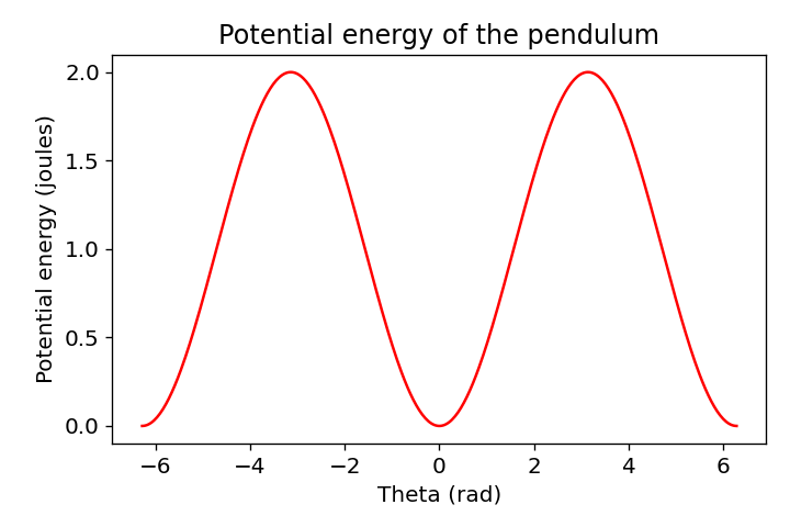
Potential energy of the pendulum (top) and phase portrait of the pendulum (bottom).

The top plot shows the potential energy of the pendulum conditional on the deflection angle $\theta$. As expected, the curve shows that the potential energy is minimal when the pendulum hangs vertically ($\theta = 0, \pm2\pi, \pm4\pi, \ldots$) and maximum when it is at the highest point of its path ($\theta = \pm\pi, \pm3\pi, \ldots$). The potential energy varies cosine-shaped with the angle $\theta$, which corresponds to the equation $U = mgl(1 - \cos(\theta))$.

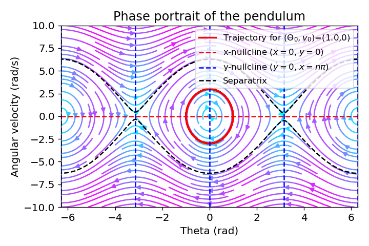
The phase portrait in the bottom plot illustrates the relationship between the deflection angle $\theta$ and the angular velocity $v = \frac{d\theta}{dt}$. The streamlines visualizes the trajectories of the pendulum in the phase plane, with each curve representing a possible motion sequence of the pendulum. The color-code indicates magnitude of the pendulum’s movement, with red indicating high speed and blue indicating low speed. The streamline’s arrows show the direction of the pendulum’s movement at each point in the phase plane. One exemplary trajectory is plotted in red, starting at the initial conditions $(\theta_0, v_0) = (1.0, 0)$. This trajectory is calculated using the solve_ivp function from the scipy.integrate module, which solves the ODE defined in the pendulum_phase_portrait function.

The Nullclines are shown as dashed lines, showing the critical points of the system, which correspond to the equilibrium positions of the pendulum. The intersections of the $\theta$- and $v$-nullclines represent the fixed points of the system. For a simple pendulum, these include the stable equilibrium point at $\theta = 0$, where the pendulum hangs directly downward, and unstable equilibrium points at $\theta = \pm \pi, \pm 2\pi, \ldots$, where the pendulum is balanced upright. At small deflections, the pendulum oscillates around the stable equilibrium point at $\theta = 0$, while larger deflections lead to more complex movements that show the periodic nature of the pendulum and the dependence of its movement on the initial conditions. Closed loops around the stable equilibrium indicate periodic oscillations and the separatrix connects the saddle points ($\theta = \pm \pi$) delineating the boundary between oscillatory and rotational motions.

The separatrix is approximated by simulating two trajectories starting near the saddle points at $(-3\pi + \epsilon, 0)$ and $(3\pi - \epsilon, 0)$, where $\epsilon$ is a small value, representing a small push to the pendulum from its unstable equilibrium position.

The phase plane plots provide valuable insights into the dynamic behaviour of the simple pendulum and its energy relationships, e.g., by varying the initial conditions:

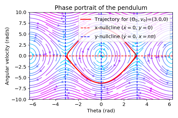
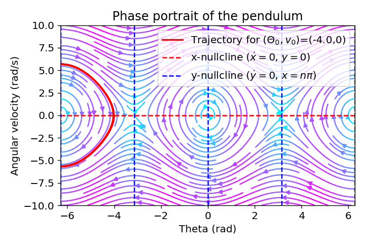Phase portrait of the pendulum with trajectories for different initial conditions.

To further analyze the local behavior of the pendulum system, we can calculate the Jacobian matrix and its eigenvalues and eigenvectors at the stable equilibrium point ($(0, 0)$) and one of the saddle points (e.g., $(\pi, 0)$). The Jacobian matrix $J$ for this system is a 2 $\times$ 2 matrix where each element is a partial derivative of the right-hand side of the equations with respect to each of the state variables ($\theta$ and $v$), evaluated at a specific point:

\[\begin{align*} J_{(\theta, v)} =& \begin{bmatrix} \frac{\partial}{\partial \theta}(\frac{d\theta}{dt}) & \frac{\partial}{\partial v}(\frac{d\theta}{dt}) \\ \frac{\partial}{\partial \theta}(\frac{dv}{dt}) & \frac{\partial}{\partial v}(\frac{dv}{dt}) \end{bmatrix} \\ =& \begin{bmatrix} 0 & 1 \\ -\frac{g}{l} \cos(\theta) & 0 \end{bmatrix} \end{align*}\]

Evaluating the Jacobian at $(\theta, v) = (0, 0)$ yields to:

\[J_{(0,0)} = \begin{bmatrix} 0 & 1 \\ -\frac{g}{l} & 0 \end{bmatrix}\]

and at $(\theta, v) = (\pi, 0)$:

\[J_{(\pi,0)} = \begin{bmatrix} 0 & 1 \\ \frac{g}{l} & 0 \end{bmatrix}\]

The eigenvalues $\lambda$ of $J$ are found by solving the characteristic equation $\det(J - \lambda I) = 0$, where $I$ is the identity matrix. To calculate the eigenvalues for our explicit points, we use $g = 9.81 \, \text{m/s}^2$ and $l = 1 \, \text{m}$ (for simplicity).

Jacobian at $(0,0)$:

$\det(J_{(0,0)} - \lambda I) = 0$ yields to:

\[\begin{vmatrix} -\lambda & 1 \\ -\frac{g}{l} & -\lambda \end{vmatrix} = \lambda^2 + \frac{g}{l} = 0\]

Solving for $\lambda$, we get:

\[\begin{align*} \lambda^2 + \frac{g}{l} =& 0 \\ \Leftrightarrow \lambda^2 =& -\frac{g}{l} \\ \Leftrightarrow \lambda =& \pm \sqrt{-\frac{g}{l}} = \pm i\sqrt{9.81} \end{align*}\]

The eigenvalues are complex and have no real part. This is indicative of the pendulum’s stable equilibrium point being a center, where the pendulum oscillates around the equilibrium point without converging or diverging.

To find the eigenvectors, substitute, e.g., $\lambda=\sqrt{-\frac{g}{l}}$ into $(J - \lambda I)v = 0$ (with $v=(x,y)$, the eigenvector):

\[\begin{align*} \left( \begin{bmatrix} 0 & 1 \\ -\frac{g}{l} & 0 \end{bmatrix} - \begin{bmatrix} i\sqrt{\frac{g}{l}} & 0 \\ 0 & i\sqrt{\frac{g}{l}} \end{bmatrix} \right) \begin{bmatrix} x \\ y \end{bmatrix} =& 0 \\ \Leftrightarrow \begin{bmatrix} -i\sqrt{\frac{g}{l}} & 1 \\ -\frac{g}{l} & -i\sqrt{\frac{g}{l}} \end{bmatrix} \begin{bmatrix} x \\ y \end{bmatrix} =& 0 \end{align*}\]

To solve the system, we can choose $x = 1$ for simplicity, leading to:

\[y = i\sqrt{\frac{g}{l}}\]

Thus, one eigenvector is \(\begin{bmatrix} 1 \\ i\sqrt{\frac{g}{l}} \end{bmatrix}\). For complex $\lambda$, the eigenvectors are also complex with no real part.

Jacobian at $(\pi,0)$:

$\det(J_{(\pi,0)} - \lambda I) = 0$ yields to:

\[\begin{vmatrix} -\lambda & 1 \\ \frac{g}{l} & -\lambda \end{vmatrix} = \lambda^2 - \frac{g}{l} = 0\]

Solving for $\lambda$, we get:

\[\begin{align*} \lambda^2 - \frac{g}{l} =& 0 \\ \Leftrightarrow \lambda =& \pm \sqrt{\frac{g}{l}} = \pm \sqrt{9.81} \end{align*}\]

Finding the eigenvectors involves again substituting, e.g., $\lambda=\frac{g}{l}$ back into $(J - \lambda I)v = 0 $:

\[\begin{align*} \left( \begin{bmatrix} 0 & 1 \\ \frac{g}{l} & 0 \end{bmatrix} - \begin{bmatrix} \sqrt{\frac{g}{l}} & 0 \\ 0 & \sqrt{\frac{g}{l}} \end{bmatrix} \right) \begin{bmatrix} x \\ y \end{bmatrix} =& 0 \\ \Leftrightarrow \begin{bmatrix} -\sqrt{\frac{g}{l}} & 1 \\ -\frac{g}{l} & -\sqrt{\frac{g}{l}} \end{bmatrix} \begin{bmatrix} x \\ y \end{bmatrix} =& 0 \end{align*}\]

To solve the system, we can again choose $x = 1$ for simplicity, leading to:

\[y = \sqrt{\frac{g}{l}}\]

Thus, one eigenvector is \(\begin{bmatrix} 1 \\ \sqrt{\frac{g}{l}} \end{bmatrix}\).

This time, the eigenvalues are real and have opposite signs, one positive ($3.132$) and one negative ($-3.132$), indicating that this point is indeed a saddle point. Trajectories near this point will be attracted along the direction of the eigenvector associated with the negative eigenvalue and repelled along the direction of the eigenvector associated with the positive eigenvalue.

These calculations demonstrate the different local behaviors at these two critical points of the pendulum’s phase space:

• at $(0, 0)$, the pendulum exhibits neutral stability with oscillatory behavior around the equilibrium.
• at $(\pi, 0)$, the pendulum’s dynamics show a clear saddle point behavior, with trajectories being repelled or attracted depending on their initial conditions relative to the eigenvectors’ directions.

Conclusion

In conclusion, phase plane analysis emerges as an important tool in the exploration of dynamical systems, offering profound insights into their behavior through a graphical representation of state variables and their interactions. This analysis facilitates a deeper understanding of complex systems that are often described by nonlinear differential equations, which can be challenging to solve analytically. By converting these systems into a set of first-order equations, phase plane analysis allows for the visualization of trajectories, equilibrium points, and limit cycles, which are instrumental in predicting system behavior over time. Moreover, the integration of nullclines and the examination of eigenvalues and eigenvectors provide a comprehensive framework for assessing stability and predicting long-term behavior.

In the context of computational neuroscience, phase plane analysis is particularly valuable for understanding the behavior of neural systems, such as the occurrence of oscillations and the emergence of limit cycles, which are crucial for many neural functions. The ability to visualize and analyze the dynamics of these systems is essential for understanding the underlying mechanisms of neural function and for developing models that accurately represent the behavior of neurons and neural networks.

The Python code used in this post is freely available in this GitHub repositoryꜛ.

References and further reading

• Chapter 4, Dimensionality reduction and phase plane analysis, from Wulfram Gerstner, Werner M. Kistler, Richard Naud, and Liam Paninski (2014), Neuronal Dynamics: From Single Neurons to Networks and Models of Cognition, Cambridge University Press, https://www.cambridge.org/9781107060838, free online versionꜛ
• Chapter 3, Phase-plane analysis: introduction, from Eric Feron and James Paduano, Estimation And Control Of Aerospace Systems, 2004, OpenCourseWare, MIT, PDFꜛ
• Wikipedia article on phase plane analysisꜛ