Van der Pol oscillator

March 24, 2024 March 29, 2024 15 minute read comments

After we have discussed the basics of phase plane analysis in the previous post, we will now apply this method to the Van der Pol oscillator. The Van der Pol oscillator is a non-conservative oscillator with nonlinear damping, which was first described by the Dutch electrical engineer Balthasar van der Pol in 1920. It was originally used to describe the behavior of electronic circuits in the first radios, but it has since been applied to a wide range of systems in physics, biology, and engineering. We will explore how phase plane analysis can be used to gain insights into the behavior of this system and how it can be used to predict its long-term behavior.

jpg

Van der Pol equation

The system is described by a second-order ODE,

\[\begin{align} \frac{d^{2}x}{dt^{2}} -\mu (1-x^{2}){dx \over dt}+x=0, \label{eq:1} \end{align}\]

where $x$ is the position of the oscillator and $\mu$ is a parameter that determines the nonlinearity and the damping of the system. The MIT lecture notes by Rothman (2022)ꜛ provide a detailed derivation of the Van der Pol equation and I recommend reading it to get a deeper understanding of the origin of the system parameters.

Using linearization

The ODE ($\ref{eq:1}$) can be converted into a system of first-order ODEs by introducing a new variable $y = \frac{dx}{dt}$:

\[\begin{align*} \dot{x} &= y, \\ \dot{y} &= \mu(1 - x^2)y - x, \end{align*}\]

The nullclines of the Van der Pol oscillator are given by the conditions under which the derivatives $\frac{dx}{dt}$ and $\frac{dy}{dt}$ are zero. The $x$-nullcline is determined by setting $\frac{dx}{dt} = 0$, which occurs when $y = 0$, i.e., this nullcline is represented by a horizontal line at $y = 0$. The $y$-nullcline is found by setting $\frac{dy}{dt} = 0$, which occurs when $\mu(1 - x^2)y - x = 0$ $\Leftrightarrow$ $y = \frac{x}{\mu(1-x^2)}$.

For certain values of $\mu$, the Van der Pol oscillator exhibits limit cycle behavior. Let’s explore this behavior by visualizing the phase plane of the Van der Pol oscillator and identifying its limit cycle:

import numpy as np
import matplotlib.pyplot as plt
from scipy.integrate import solve_ivp

# define the Van der Pol oscillator model:
def van_der_pol(t, z, mu):
    x, y = z
    dxdt = y
    dydt = mu * (1 - x**2) * y - x
    return [dxdt, dydt]

# define the nullclines:
def y_nullcline(x, mu):
    return x/(mu*(1-x**2))
def x_nullcline(y, mu):
    return 0*y

# set time span:
eval_time = 100
t_iteration = 1000
t_span = [0, eval_time]
t_eval = np.linspace(*t_span, t_iteration)

# set initial conditions:
z0 = [2, 0]

# set Van der Pol oscillator parameter:
mu = 1 # stable: 1

# calculate the vector field:
mgrid_size = 8
x, y = np.meshgrid(np.linspace(-mgrid_size, mgrid_size, 15), 
                   np.linspace(-mgrid_size, mgrid_size, 15))
u = y
v = mu * (1 - x**2) * y - x

# calculating the trajectory for the Van der Pol oscillator:
sol_stable = solve_ivp(van_der_pol, t_span, z0, args=(mu,), t_eval=t_eval)

# define the x-array for the nullclines:
x_null = np.arange(-mgrid_size,mgrid_size,0.001)

# plot vector field and trajectory:
plt.figure(figsize=(6, 6))
plt.clf()
speed = np.sqrt(u**2 + v**2)
plt.streamplot(x, y, u, v, color=speed, cmap='cool', density=2.0)
plt.plot(x_null, y_nullcline(x_null, mu)  , '.', c="darkturquoise", markersize=2)
plt.plot(x_null, x_nullcline(x_null, mu)  , '.', c="darkturquoise", markersize=2)
plt.plot(sol_stable.y[0], sol_stable.y[1], 'r-', lw=3,
         label=f'Trajectory for $\mu$={mu}\nand $z_0$={z0}')  # trajectory
# indicate start point:
plt.plot(sol_stable.y[0][0], sol_stable.y[1][0], 'bo', label='start point', alpha=0.75, markersize=7)
plt.plot(sol_stable.y[0][-1], sol_stable.y[1][-1], 'o', c="yellow", label='end point', alpha=0.75, markersize=7)
plt.title('phase plane plot: Van der Pol oscillator')
plt.xlabel('x')
plt.ylabel('y')
plt.legend(loc='lower right') #, bbox_to_anchor=(1, 0.5)
plt.gca().spines['top'].set_visible(False)
plt.gca().spines['right'].set_visible(False)
plt.gca().spines['bottom'].set_visible(False)
plt.gca().spines['left'].set_visible(False)
plt.ylim(-mgrid_size, mgrid_size)
plt.tight_layout()
plt.show()

The code above generates a phase plane plot of the Van der Pol oscillator for a given set of initial conditions z0 ($=(x_0,y_0)$) and a parameter $\mu$. The trajectory is represented by the red curve and its starting and end point are indicated by blue and yellow dots, respectively. The nullclines are plotted in cyan, and the vector field is represented by the color-coded streamlines. To understand the dynamics of the system, we can change the initial conditions and the parameter $\mu$ to see how the system’s behavior changes.

Let’s start with a stable limit cycles by setting $\mu=1$:

Phase plane plot for the Van der Pol oscillator with $\mu=1$ and different initial conditions: z0=[2, 0], z0=[0.01, 0], z0=[7, 1], and z0=[-7, 1].

For $\mu=1$, the phase plane plot show, that the system converges to a closed limit cycle for all four initial conditions. The vector field indicates that the system’s trajectories are attracted to the limit cycle. Near the origin (z0=[0.01, 0]), the system is unstable with a spiral sink behavior, but evolves to the limit cycle. Far from the origin (z0=[7, 1] and z0=[-7, 1]), the system is damped, but also evolves to the limit cycle.

The $y$-nullcline intersects the $x$-axis at $x = 0$ and approaches the vertical asymptotes at $x = \pm1$, which corresponds to the points where the denominator becomes zero and the dynamics of the system become strongly nonlinear. The shape of the $y$-nullcline helps to understand the regions in the phase plane where the rate of change of the $y$-variable (represented by the motion in the $y$-direction) increases or decreases, which is crucial for analyzing the stability and dynamic behavior of the system.

In general, for all initial conditions with $\mu\gt0$, the system converges to a globally stable limit cycle:

Phase plane plot for the Van der Pol oscillator for the initial condition z0=[4, 0], and with $\mu=0$, $\mu=1$, $\mu=2$, and $\mu=4$.

For $\mu=0$, there is no damping and the system becomes a form of a simple harmonic oscillator.

For negative values of $\mu$, the system exhibits unstable behavior and the trajectories diverge from the origin:

Phase plane plot for the Van der Pol oscillator for the initial condition z0=[2.25, 0] and with $\mu=-2$.

How to interpret our findings? The graphical analysis of the phase plane plots allows us to identify parameter values of $\mu$, which lead to a stable oscillatory behavior of the Van der Pol oscillator. It also allows us to identify the stability of the limit cycle and the system’s behavior for different initial conditions. This information is crucial for understanding the dynamic properties of the Van der Pol oscillator and its behavior in different parameter regimes.

Applying a Liénard transformation

Another approach to analyze the Van der Pol oscillator is to transform it into a Liénard system. A Liénard equation is a second-order differential equation of the form

\[{d^{2}x \over dt^{2}}+f(x){dx \over dt}+g(x)=0\]

with $f(x)$ and $g(x)$ being continuously differentiable functions on $\mathbb{R}$, where $f$ is an even function and $g$ is an odd function. The Van der Pol oscillator is such a system with $f(x) = -\mu(1-x^2)$ and $g(x) = x$. The advantage of the Liénard equation is that, by applying an appropriate transformation by introducing a new variable, it can be reduced to a first-order system of ODEs, which can be analyzed more easily.

The commonly used Liénard transformation for the Van der Pol oscillator is given by defining a new variable $y=x-x^{3}/3-{\dot {x}}/\mu$, that combines $x$, $\dot{x}$, and a non-linear term of $x$. The transformation is tailored to both linearize parts of the system and clearly separate the dynamics into two interacting parts. Using this transformation, we differentiate $y$ with respect to $t$ to connect it to the original equation:

\[\dot{y} = \dot{x} - x^2\dot{x} - \frac{1}{\mu}\ddot{x}.\]

Substituting $\ddot{x}$ from the Van der Pol equation gives us:

\[\dot{y} = \dot{x} - x^2\dot{x} + (1-x^2)\dot{x} - \frac{x}{\mu} = -\frac{x}{\mu},\]

which simplifies based on the cancellation of terms. Therefore, the transformation leads to the following two first-order differential equations:

\[\begin{align*} \dot{x} &= \mu \left(x-{\tfrac {1}{3}}x^{3}-y\right), \\ \dot{y} &= {\frac {1}{\mu }}x. \end{align*}\]

The $\dot{x}$ equation is derived by rearranging the terms of the $y$ transformation term. The system is now in a form suitable for phase plane analysis, numerical simulation, and further analytical study. The corresponding $\dot{x}=0$ and $\dot{y}=0$-nullclines are

\[\begin{align*} & \dot{x}=0 \\ \Leftrightarrow \; & \mu \left(x - \frac{1}{3}x^3 - y\right) = 0 \\ \Leftrightarrow \; & y = x - \frac{1}{3}x^3 \end{align*}\]

and

\[\begin{align*} \dot{y}=0 \Leftrightarrow \; & \frac{1}{\mu}x = 0 \end{align*}\]

The $\dot{x}=0$-nullcline is a cubic function and the $\dot{y}=0$-nullcline is a vertical line through the origin.

The transformed ODE and its nullclines do indeed look different from the ones we have derived above, which can lead to variations in the qualitative depiction of the dynamics on the phase plane. However, this difference does not necessarily contradict the equivalence of both transformations in capturing the dynamical behavior of the original equation. The primary goal of both transformations is to make the analysis of the original system more tractable. Each does so by unpacking the oscillator’s dynamics into a format that is easier to analyze. While the nullclines are indeed different between the two transformed systems, each set of nullclines provides unique insights into the oscillator’s behavior. The first-order system transformation directly translates the original dynamics into a two-dimensional phase plane, making the oscillator’s limit cycle behavior directly observable. The Liénard transformation, on the other hand, restructures the dynamics to highlight the energy exchange and damping effects in a different but equivalently valid two-dimensional representation. The difference in nullclines and the resulting phase portraits does not imply a contradiction but rather reflects different perspectives on the same dynamical phenomena. The core dynamical behavior — the presence of self-sustained oscillations and how they are affected by the non-linearity parameter $\mu$ — remains consistent across both representations and the original system, as we will see in the following.

Our previous Python code can be easily adapted to visualize the phase plane of the Van der Pol oscillator using the Liénard transformation. Simply modify the van_der_pol function to represent the Liénard system and adjust the nullclines accordingly. The according code can be found in the Github repository mentioned below.

Let’s interpret the results:

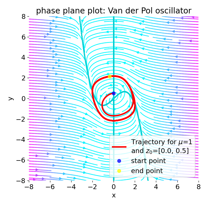
Phase plane plot for the Van der Pol oscillator (using Liénard transformation) with $\mu=1$ and different initial conditions: z0=[0, 0.5], z0=[4, 0], z0=[4, -4], and z0=[0, 0].

With $\mu=1$, the phase plane plot shows that the system converges to a closed limit cycle for different initial conditions. The vector field indicates that the system’s trajectories are attracted always to the limit cycle. Near the origin (z0=[0, 0.5]), the system is again unstable with a spiral sink behavior, but evolves to the limit cycle. Far from the origin (z0=[4, 0] and z0=[4, -4]), the system is damped, but also evolves to the limit cycle. When the trajectory starts exactly at the origin (z0=[0, 0]), no oscillations are observed, which is consistent with the fact that the origin is a stable equilibrium point for the Liénard system.

Phase plane plot for the Van der Pol oscillator for the initial condition z0=[2, 0], and with $\mu=1$, $\mu=2$, $\mu=4$, and $\mu=8$.

For increasing values of $\mu\gt1$, limit cycle becomes smaller and the system’s behavior becomes more damped. This leads to faster convergence to the limit cycle and a decrease in the amplitude of the oscillations.

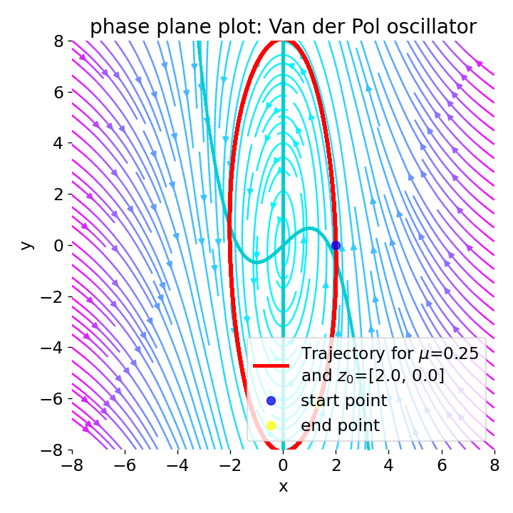Phase plane plot for the Van der Pol oscillator for the initial condition z0=[2, 0], and with $\mu=0.5$, and $\mu=0.25$.

For $0\lt\mu\lt1$, the system still exhibits stable limit cycle behavior, but the limit cycle becomes larger and the system’s behavior becomes less damped. This leads to slower convergence to the limit cycle and an increase in the amplitude of the oscillations. Note, that for $\mu=0$, no solution can be derived this time as we would have a division by zero in the Liénard transformation.

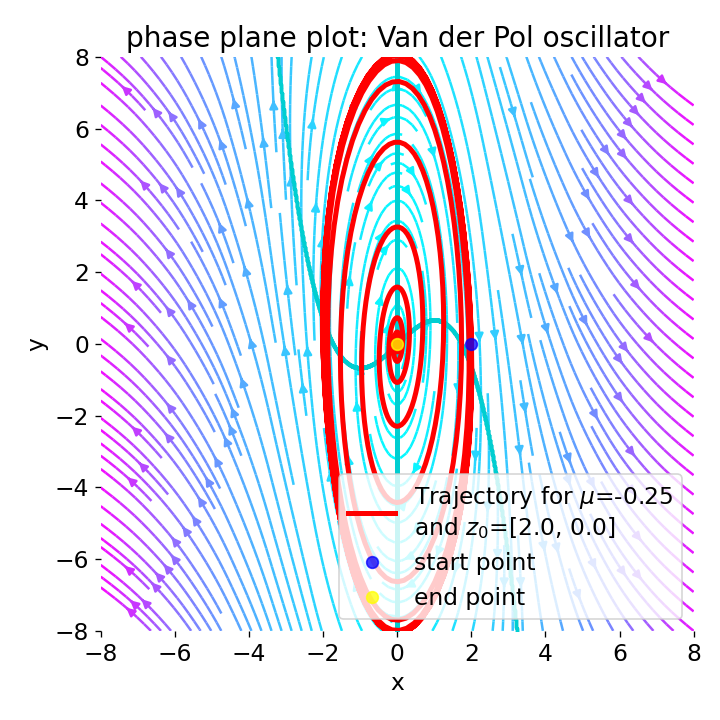
Phase plane plot for the Van der Pol oscillator for different initial conditions and with $\mu=\lt0$.

For negative values of $\mu$, the system exhibits unstable behavior. A negative $\mu$ alters the nature of the damping in the system. Instead of the non-linear damping that stabilizes the limit cycle for positive $\mu$, negative $\mu$ values can lead to an increase in the system’s energy, potentially destabilizing it or altering its convergence behavior.

Depending on the initial conditions, the system either converges to a stable equilibrium point or the trajectories diverge from the origin. Whether the system converges to a stable equilibrium point or the trajectories diverge from the origin depends on whether the initial conditions lie with respect to the $\dot{x}=0$-nullcline. The $\dot{x}=0$ nullcline effectively represents points in the phase space where the horizontal (x-direction) velocity component is zero. The system’s behavior on either side of this nullcline is determined by the sign and magnitude of $\dot{y}$, which, in combination with the effects of $\mu$, influences whether trajectories move towards or away from the nullcline and potentially cross it. The position of the initial condition relative to this nullcline helps to determine the trajectory’s initial direction and behavior, influencing convergence or divergence outcomes.

And again, the larger the absolute value of $\mu$, the faster the convergence to the stable equilibrium point. The magnitude of $\mu$ indeed affects the rate at which trajectories converge to any stable points or diverge. Larger absolute values of $\mu$ tend to result in faster dynamics, either hastening the convergence to equilibrium points or accelerating the divergence from unstable points.

In order to further analyze the fix points and the stability of the system, we can again use the Jacobian matrix and its eigenvalues. The Jacobian matrix of the Liénard system is given by

\[J = \begin{bmatrix} \frac{\partial \dot{x}}{\partial x} & \frac{\partial \dot{x}}{\partial y} \\ \frac{\partial \dot{y}}{\partial x} & \frac{\partial \dot{y}}{\partial y} \end{bmatrix} = \begin{bmatrix} \mu(1 - x^2) & -\mu \\ \frac{1}{\mu} & 0 \end{bmatrix}.\]

Evaluating the Jacobian at the fixed point $(0,0)$ gives:

\[J(0,0) = \begin{bmatrix} \mu & -\mu \\ \frac{1}{\mu} & 0 \end{bmatrix}.\]

The eigenvalues $\lambda$ of the Jacobian matrix are found by solving the characteristic equation

\[\det(J - \lambda I) = 0,\]

where $I$ is the identity matrix.

For the given $J(0,0)$, the characteristic equation becomes:

\[\begin{vmatrix} \mu - \lambda & -\mu \\ \frac{1}{\mu} & -\lambda \end{vmatrix} = 0.\]

Solving this equation will give us the eigenvalues:

\[\lambda = \frac{\mu}{2} - \frac{\sqrt{\mu^2 - 4}}{2}, \quad \frac{\mu}{2} + \frac{\sqrt{\mu^2 - 4}}{2}.\]

Let’s analyze what the eigenvalues tell us about the system’s behavior in case of small perturbations around the fixed point $(0,0)$ and how the system’s stability depends on the parameter $\mu$:

for $\mu \gt 2$: When $\mu \gt 2$, the term under the square root, $\mu^2 - 4$, is positive, leading to real and distinct eigenvalues. Since the value of $\mu/2$ is positive, the sign of the real parts of the eigenvalues depends on the value of $\mu$. Both eigenvalues have positive real parts, given that adding or subtracting a positive square root to/from a positive $\mu/2$ keeps the sign positive. This indicates that the fixed point is indeed an unstable node, as all trajectories move away from it.
for $0 \lt \mu \lt 2$: In this range, the term under the square root becomes negative ($\mu^2 - 4 < 0$), which means the eigenvalues are complex with real parts given by $\mu/2$, and imaginary parts determined by the square root of a negative number. Since the real part of the eigenvalues ($\mu/2$) is positive for any $\mu > 0$, the fixed point is an unstable spiral, not a node, implying that trajectories spiral out from the fixed point.
for $-2 \lt \mu \lt 0$: In this range, the term under the square root is still negative, leading to complex eigenvalues with real parts given by $\mu/2$. Since $\mu/2$ is negative in this case, the fixed point is a stable spiral, implying that trajectories spiral in towards the fixed point.
for $|\mu| = 2$: The term under the square root is zero, resulting in a repeated real eigenvalue $\mu/2$. This is a special case indicating a bifurcation point where the nature of the fixed point can change. A bifurcation occurs when the system’s behavior changes qualitatively as a parameter is varied. In this case, the fixed point is critically stable and the system is on the verge of instability. For $\mu = 2$, the eigenvalue is positive, suggesting a critically stable case that is on the verge of instability. For $\mu = -2$, the eigenvalue is negative, indicating a critically stable case that is on the verge of stability.
for $\mu \lt - 2$: When $\mu < -2$, the term under the square root, $\mu^2 - 4$, is again positive, resulting in real and distinct eigenvalues. Since $\mu/2$ is negative, and the square root term affects the magnitude without changing the sign, both eigenvalues are negative. This means that the fixed point is a stable node, with trajectories moving toward it from all directions.

Physical interpretation

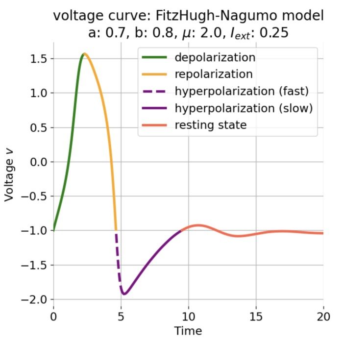
To understand what it means, when the system converges to a stable limit cycle, we can examine its $x(t)$ component. For instance, below are two plots of $x(t)$, one for $\mu=-1$ and z0=[1.0, 0.0] (top), and another one for $\mu=2$ and z0=[0.5, 0.5] (bottom):

Top: Phase plane plot and corresponding $x(t)$ component of the Van der Pol oscillator for $\mu=-1$ and z0=[1.0, 0.0]. Bottom: Analogous plot for $\mu=2$ and z0=[0.5, 0.5].

In the first case (top plot), the system does not converge to a stable limit cycle. After an initial swing, the system converges rapidly to a stable equilibrium point ($0$). In the second case (bottom plot), the system converges to a stable limit cycle and the $x(t)$ component oscillates around the equilibrium point. Convergence to a stable limit cycle means that the system exhibits a self-sustained oscillation that persists over time. Furthermore, the limit cycle is a stable attractor, where the trajectories are attracted to the limit cycle and remain there over time, regardless of the chosen initial conditions. The limit cycle is a characteristic feature of the Van der Pol oscillator and represents the system’s long-term behavior.

Conclusion

In this post, we have applied phase plane analysis to the Van der Pol oscillator. We have visualized the phase plane of the Van der Pol oscillator and identified its limit cycle for different initial conditions and parameter values. We have also discussed the influence of the Liénard transformation on the phase plane and the system’s dynamics. The graphical analysis of the phase plane plots has allowed us to identify parameter values of $\mu$ that lead to a stable oscillatory behavior and those that lead to unstable behavior. We have also identified the stability of the limit cycle and the system’s behavior for different initial conditions. This information is crucial for understanding the dynamic properties of the Van der Pol oscillator and its behavior in different parameter regimes. The phase plane analysis has again provided us with a powerful tool to gain insights into the behavior of a dynamical system and to predict its long-term behavior.

You can find the complete code used in this post in this GitHub repositoryꜛ.