Incorporating structural plasticity in neural network models
In standard spiking neural networks (SNN), synaptic connections between neurons are typically fixed or change only according to specific plasticity rules, such as Hebbian learning or Spike-Timing Dependent Plasticity (STDP). However, the brain’s connectivity is not static. Neurons can grow and retract synapses in response to activity levels and environmental conditions. A phenomenon known as structural plasticity. This process plays a crucial role in learning and memory formation in the brain. To illustrate how structural plasticity can be modeled in spiking neural networks, in this post, we will use the NEST Simulator and replicate the tutorial on “Structural Plasticity”ꜛ.
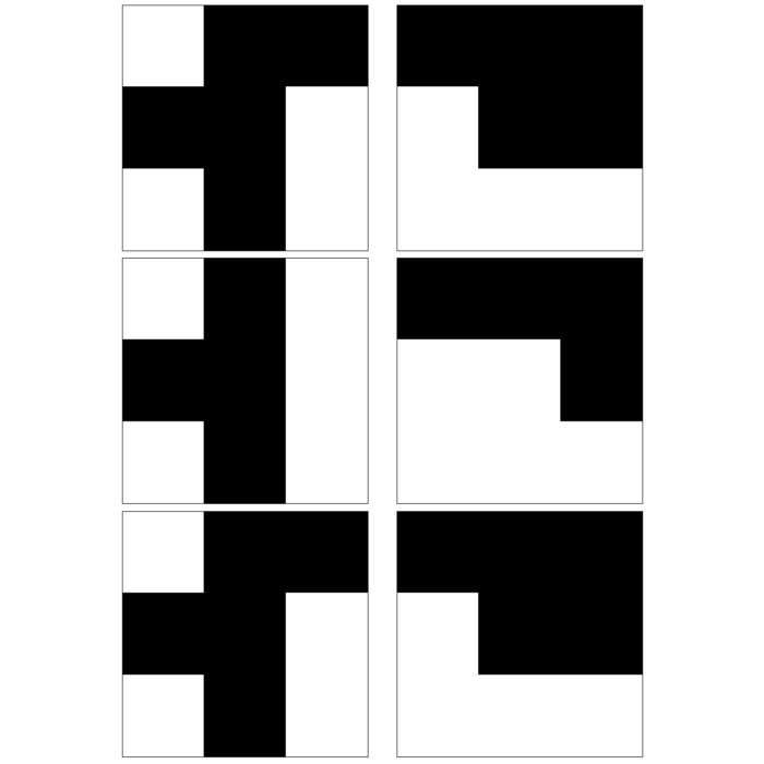
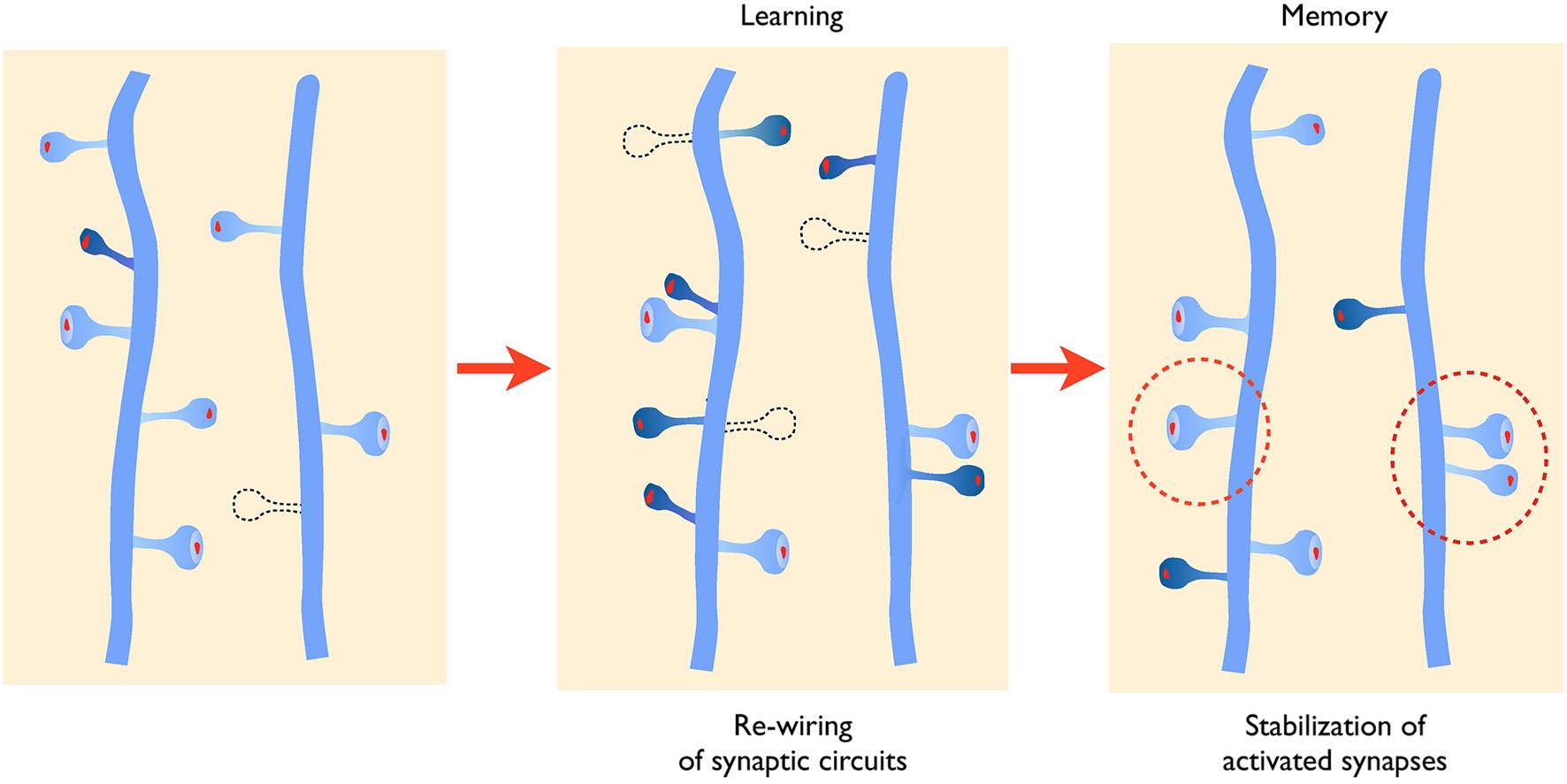 Sketch illustrating structural plasticity during learning and memory formation. The sketch illustrates the dynamic remodeling of synaptic connectivity through dendritic spine turnover. Left: Under baseline conditions, synaptic networks exhibit continuous formation and elimination of dendritic spines, reflecting ongoing structural plasticity. Middle: During learning or learning related activity, this baseline turnover is transiently increased, leading to enhanced formation and pruning of synaptic contacts. Newly formed spines preferentially emerge near previously activated synapses, promoting the local clustering of synaptic inputs and enabling adaptive rewiring of circuits. Right: A subset of newly formed and activated synapses becomes selectively stabilized, providing a structural substrate for the long term retention of behaviorally relevant connections and memory traces. Source: Bernardinelli, Y., Nikonenko, I., Muller, D., Structural plasticity: mechanisms and contribution to developmental psychiatric disorders, Frontiers in Neuroanatomy, 2014, 8:123, doi 10.3389/fnana.2014.00123ꜛ (license: CC BY 4.0).
What is structural plasticity?
Structural plasticity refers to the ability of neurons to change their physical structure by forming new synaptic connections or eliminating existing ones. This plasticity is crucial for the brain’s ability to adapt to new experiences, learn, and recover from injuries. Structural plasticity involves several processes, including:
- Synaptogenesis: The formation of new synapses
- Synaptic pruning: The elimination of less active or redundant synapses
- Dendritic growth and retraction: Changes in the length and branching of dendrites
- Axonal sprouting: The growth of new axonal branches to form new synapses
How structural plasticity is modeled in SNNs
To model structural plasticity in SNNs, we incorporate mechanisms that allow neurons to add or remove synaptic elements based on specific rules. These elements, called synaptic elements, include (presynaptic) axonal boutons and (postsynaptic) dendritic spines. The growth and pruning of these elements are governed by growth curves, which are functions that determine the rate of growth or retraction based on factors such as calcium concentration in the neurons.
The main difference between standard SNNs and those incorporating structural plasticity lies in the dynamic nature of the network’s connectivity. In a standard SNN, synaptic connections are often fixed or modified only by local plasticity rules like Spike-Timing Dependent Plasticity (STDP). In contrast, a structurally plastic network can create and remove connections based on global network activity, thereby simulating more realistic brain-like adaptability.
NEST simulation
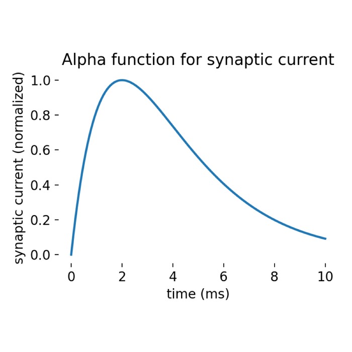
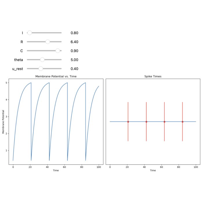
To illustrate structural plasticity in spiking neural networks, we will replicate the NEST tutorial “Structural Plasticity example”ꜛ including some minor modifications. We will use NEST’s iaf_psc_alphaꜛ neuron model which is a leaky integrate-and-fire neuron (LIF) model with post-synaptic current shaped as an alpha function. The tutorial reproduces the results shown in Butz and van Ooyen (2013)ꜛ. All parameters and growth curves are defined according to this publication.
The model consists of 800 excitatory and 200 inhibitory neurons. Initially, no connections exist between the neurons. The network is stimulated with a Poisson input, and the connectivity is updated based on homeostatic rules defined as growth curves for synaptic elements. According to these rules, structural plasticity will create and delete synapses dynamically during the simulation until a desired level of activity is reached. The growth curves for axonal boutons and dendritic spines are defined based on the calcium concentration in the neurons. We also record the calcium concentration in the neurons and the connectivity over time to visualize the network’s structural changes.
Let’s begin with importing all necessary libraries:
import os
import matplotlib.pyplot as plt
import numpy as np
import nest
import nest.raster_plot

# Set global properties for all plots
plt.rcParams.update({'font.size': 12})
plt.rcParams["axes.spines.top"]    = False
plt.rcParams["axes.spines.bottom"] = False
plt.rcParams["axes.spines.left"]   = False
plt.rcParams["axes.spines.right"]  = False
Next, we define the simulation parameters. Note, that the implementation of structural plasticity in NEST can not be used with multiple threads (thus don’t try to increase the number of (local) threads):
# set simulation parameters:
t_sim = 200000.0 # simulation time in ms
dt = 0.1 # simulation resolution in ms (is also the resolution
         # of the update of the synaptic elements/structural plasticity)
number_excitatory_neurons = 800 # number of excitatory neurons
number_inhibitory_neurons = 200 # number of inhibitory neurons
update_interval = 10000.0 # i.e., define how often the connectivity is updated inside the network
                          # synaptic elements and connections change on different time scales
record_interval = 1000.0
bg_rate = 10000.0 # background rate (i.e. rate of Poisson sources)

nest.ResetKernel()
nest.set_verbosity("M_ERROR")
nest.resolution = dt
nest.structural_plasticity_update_interval = update_interval
For the postsynaptic currents, we define the following values:
# initialize variables for postsynaptic currents:
psc_e   = 585.0 # excitatory postsynaptic current in pA
psc_i   = -585.0 # inhibitory postsynaptic current in pA
psc_ext = 6.2 # external postsynaptic current in pA
Next, we define the neuron model parameters:
# define neuron model parameters:
neuron_model = "iaf_psc_exp"
model_params = {
    "tau_m": 10.0,      # membrane time constant (ms)
    "tau_syn_ex": 0.5,  # excitatory synaptic time constant (ms)
    "tau_syn_in": 0.5,  # inhibitory synaptic time constant (ms)
    "t_ref": 2.0,       # absolute refractory period (ms)
    "E_L": -65.0,       # resting membrane potential (mV)
    "V_th": -50.0,      # spike threshold (mV)
    "C_m": 250.0,       # membrane capacitance (pF)
    "V_reset": -65.0    # reset potential (mV)
}
Now, we define the structural plasticity properties and growth curves for the synaptic elements:
# copy synaptic models (will be the base for our structural plasticity synapses):
nest.CopyModel("static_synapse", "synapse_ex")
nest.SetDefaults("synapse_ex", {"weight": psc_e, "delay": 1.0})
nest.CopyModel("static_synapse", "synapse_in")
nest.SetDefaults("synapse_in", {"weight": psc_i, "delay": 1.0})

# define structural plasticity properties:
nest.structural_plasticity_synapses = {
        "synapse_ex": {
        "synapse_model": "synapse_ex",
        "post_synaptic_element": "Den_ex",
        "pre_synaptic_element": "Axon_ex"},
        "synapse_in": {
        "synapse_model": "synapse_in",
        "post_synaptic_element": "Den_in",
        "pre_synaptic_element": "Axon_in"}}
The structural_plasticity_synapsesꜛ method defines which synapses are subject to structural plasticity and specifies the corresponding synaptic models and elements. For each synapse type (excitatory and inhibitory), a separate dictionary is created with the synaptic model, postsynaptic element, and presynaptic element. We created a copy of the static synapse model for excitatory and inhibitory synapses and set the default weight and delay values (individually for excitatory and inhibitory synapses). These models, synapse_ex and synapse_in, will be used as the base for the structural plasticity synapses. The postsynaptic and presynaptic elements are defined as dendritic (Den_ex, Den_in) and axonal (Axon_ex, Axon_in) elements, respectively. They will be associated with the growth curves for synaptic elements in the next step.
The growth curves define the rate of growth or retraction of synaptic elements based on the calcium concentration in the neurons. The growth_rate parameter determines the speed of growth, while eps specifies the threshold calcium concentration at which growth occurs. The continuous parameter indicates whether growth is continuous or discrete. In this example, we use a Gaussian growth curve with a fixed growth rate and threshold:
# define growth curves for synaptic elements:
growth_curve_e_e = {"growth_curve": "gaussian", "growth_rate": 0.0001, "continuous": False, "eta": 0.0, "eps": 0.05}
growth_curve_e_i = {"growth_curve": "gaussian", "growth_rate": 0.0001, "continuous": False, "eta": 0.0, "eps": 0.05}
growth_curve_i_e = {"growth_curve": "gaussian", "growth_rate": 0.0004, "continuous": False, "eta": 0.0, "eps": 0.2}
growth_curve_i_i = {"growth_curve": "gaussian", "growth_rate": 0.0001, "continuous": False, "eta": 0.0, "eps": 0.2}

# define synaptic elements:
synaptic_elements   = {"Den_ex": growth_curve_e_e,
                       "Den_in": growth_curve_e_i,
                       "Axon_ex": growth_curve_e_e}
synaptic_elements_i = {"Den_ex": growth_curve_i_e,
                       "Den_in": growth_curve_i_i,
                       "Axon_in": growth_curve_i_i}
Next, we create the nodes (neurons) and connect them with a Poisson generator, which drives the network with external input:
# create_nodes:
nodes_e = nest.Create("iaf_psc_alpha", number_excitatory_neurons,
                      params={"synaptic_elements": synaptic_elements})
nodes_i = nest.Create("iaf_psc_alpha", number_inhibitory_neurons,
                      params={"synaptic_elements": synaptic_elements_i})

# create a Poisson generator for external input and make connections:
noise = nest.Create("poisson_generator", params={"rate": bg_rate})
nest.Connect(noise, nodes_e, syn_spec={"weight": psc_ext, "delay": 1.0})
nest.Connect(noise, nodes_i, syn_spec={"weight": psc_ext, "delay": 1.0})
We also define two helper functions to record the calcium concentration and connectivity in each population over time:
# create some lists to store results:
mean_ca_e = [] # mean calcium concentration of excitatory neurons
mean_ca_i = [] # mean calcium concentration of inhibitory neurons
total_connections_e = [] # total number of connections of excitatory neurons
total_connections_i = [] # total number of connections of inhibitory neurons

# define a function for recording the calcium concentration of all neurons:
def record_ca():
    global mean_ca_e, mean_ca_i
    ca_e = nest.GetStatus(nodes_e, "Ca")
    ca_i = nest.GetStatus(nodes_i, "Ca")
    # we only record the mean calcium concentration of the neurons:
    mean_ca_e.append(np.mean(ca_e))
    mean_ca_i.append(np.mean(ca_i))

# define a function for recording the number of connections:
def record_connectivity():
    """
    We retrieve the number of connected pre-synaptic elements of each neuron.
    The total amount of excitatory connections is equal to the total amount of
    connected excitatory pre-synaptic elements. The same applies for inhibitory
    connections.
    """
    global total_connections_e, total_connections_i
    syn_elems_e = nest.GetStatus(nodes_e, "synaptic_elements")
    syn_elems_i = nest.GetStatus(nodes_i, "synaptic_elements")
    total_connections_e.append(sum(neuron["Axon_ex"]["z_connected"] for neuron in syn_elems_e))
    total_connections_i.append(sum(neuron["Axon_in"]["z_connected"] for neuron in syn_elems_i))
Finally, we simulate the network and record the calcium concentration and connectivity over time. This will take some time to complete; a progress indicator is printed every 20 simulation steps:
# simulate:
nest.EnableStructuralPlasticity()
print("Starting simulation...")
sim_steps = np.arange(0, t_sim, record_interval)
for i, step in enumerate(sim_steps):
    nest.Simulate(record_interval)
    record_ca()
    record_connectivity()
    if i % 20 == 0:
        print(f"  progress: {i / 2}%")
print("...simulation finished.")
For visualization, we plot the mean calcium concentration and connectivity over time:
# plots:
fig, ax1 = plt.subplots(figsize=(6, 4.5))
ax1.plot(mean_ca_e, "b", label="Ca concentration excitatory Neurons", linewidth=2.0)
ax1.plot(mean_ca_i, "r", label="Ca concentration inhibitory Neurons", linewidth=2.0)
ax1.axhline(growth_curve_i_e["eps"], linewidth=4.0, color="#FF9999") # plot the growth curve for inhibitory neurons
ax1.axhline(growth_curve_e_e["eps"], linewidth=4.0, color="#9999FF") # plot the growth curve for excitatory neurons
ax1.set_ylim([0, 0.28])
ax1.set_xlabel("time in [s]")
ax1.set_ylabel("Ca concentration")
ax1.legend(loc='upper right')

ax2 = ax1.twinx()
ax2.plot(total_connections_e, "m", label="excitatory connections", linewidth=2.0, linestyle="--")
ax2.plot(total_connections_i, "k", label="inhibitory connections", linewidth=2.0, linestyle="--")
ax2.set_ylim([0, 2500])
ax2.set_ylabel("Connections")
ax2.legend(loc='lower right')
plt.tight_layout()
plt.savefig("figures/structural_plasticity.png", dpi=200)
plt.show()
Results
Let’s have a look at the simulation results:
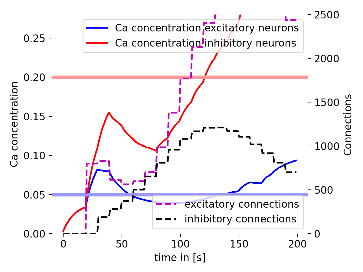 Simulation results of the structural plasticity model. The plot shows the temporal evolution of the mean calcium concentration of excitatory and inhibitory neurons (blue and red lines, respectively) and the total number of connections of excitatory and inhibitory neurons (magenta and black dashed lines, respectively). The horizontal lines represent the growth curves for excitatory (blue) and inhibitory (red) neurons. The model demonstrates how the network’s connectivity changes over time based on the calcium concentration in the neurons. The growth curves determine the threshold at which synapses are created or pruned.
The plot shows the evolution of calcium concentration and the number of synaptic connections over time. The blue and red lines represent the mean calcium concentration of excitatory and inhibitory neurons, respectively. The magenta and black dashed lines show the total number of connections of excitatory and inhibitory neurons. The horizontal lines show the target calcium concentration for excitatory neurons (blue) and inhibitory neurons (red) from growth curve parameters. The model demonstrates how the network’s connectivity changes over time based on the calcium concentration in the neurons.
Calcium concentration
The calcium concentration of the excitatory neurons starts low and gradually increases, showing some fluctuations around the target level. It suggests that the excitatory neurons are adjusting their synaptic elements in response to the calcium dynamics to maintain homeostasis (i.e., the desired level of activity).
The calcium concentration in inhibitory neurons also starts low but increases more rapidly compared to excitatory neurons. This rapid increase indicates strong synaptic activity and adjustment in inhibitory neurons. However, the calcium concentration does not stabilize at the target level, but continues to further increase, suggesting a more dynamic regulation in inhibitory neurons.
Number of connections
The number of excitatory connections increases steadily with some fluctuations, reflecting synaptic growth driven by structural plasticity. The growth seems to slow down and turning into a decay phase after reaching a certain level at the end of the simulation.
The calcium concentration in inhibitory neurons also starts low but increases more rapidly compared to excitatory neurons. This rapid increase indicates strong synaptic activity and adjustment in inhibitory neurons. Unlike the excitatory neurons, the calcium concentration does not stabilize at the target level but continues to rise, suggesting a more dynamic regulation in inhibitory neurons.
Interpretation:
- Homeostatic plasticity: The calcium concentration approaching their respective target levels (horizontal lines) illustrate the homeostatic regulation of synaptic elements. This mechanism ensures that neurons maintain a stable level of activity over time.
- Synaptic growth and retraction: The increase and subsequent decay in the number of connections (both excitatory and inhibitory) indicate synaptic growth and retraction driven by structural plasticity. The dynamic nature of these changes is crucial for maintaining calcium homeostasis and overall network stability.
- Structural plasticity dynamics: The plot highlights the dynamics of structural plasticity, where neurons continuously adjust their synaptic connections to maintain calcium homeostasis. This adjustment is vital for network stability and functionality.
- Excitatory vs. inhibitory dynamics: The difference in growth rates between excitatory and inhibitory connections, with excitatory connections showing a more pronounced increase and later decay, reflects the different roles and dynamics of these types of neurons in the network. Excitatory neurons tend to have more dynamic growth phases, while inhibitory neurons show a more balanced and regulated adjustment.
Conclusion
Incorporating structural plasticity in neural network models allows us to simulate the dynamic changes in synaptic connections observed in the brain. By modeling the growth and pruning of synaptic elements based on calcium concentration and growth curves, we can capture the adaptive nature of neural networks and their ability to reorganize in response to activity levels. The simulation results demonstrate how structural plasticity drives the formation and elimination of synapses, maintaining network stability and homeostasis. This approach provides insights into the mechanisms underlying learning, memory formation, and network plasticity in the brain.
The complete code used in this blog post is available in this Github repositoryꜛ (structural_plasticity.py). Feel free to modify and expand upon it, and share your insights.
References
- Markus Butz, Arjen van Ooyen, A Simple Rule for Dendritic Spine and Axonal Bouton Formation Can Account for Cortical Reorganization after Focal Retinal Lesions, 2013, PLoS Computational Biology, Vol. 9, Issue 10, pages e1003259, doi: 10.1371/journal.pcbi.1003259ꜛ
- NEST’s tutorial “Structural Plasticity example”ꜛ
- NEST’s
iaf_psc_alphamodel descriptionꜛ - NEST’s
structural_plasticity_synapsesmethodꜛ - Bernardinelli, Y., Nikonenko, I., Muller, D., Structural plasticity: mechanisms and contribution to developmental psychiatric disorders, 2014, Frontiers in Neuroanatomy, 8:123, doi 10.3389/fnana.2014.00123ꜛ


comments