Neural plasticity and learning: A computational perspective

February 2, 2026 30 minute read see also comments

After having discussed structural plasticity in some detail in the previous post, I thought it would be useful to take now a broader look at neural plasticity and learning from a computational perspective. Both, plasticity and learning are fundamental adaptive processes that enable the brain to modify its structure and function in response to experience. But what are the main forms of plasticity, how do they relate to learning, and how can we formalize these concepts in models of neural dynamics? In this post, I will explore these questions, based on my so-far understanding of the topic. As in all areas of science, these views are subject to ongoing revision as new data and theoretical frameworks emerge and as my own understanding develops. I will update this post accordingly over time. Please keep that in mind while reading. If you find something that is inaccurate, incomplete, or misleading, please let me know in the comments below. For a more comprehensive treatment, I recommend consulting the references listed at the end of the post.

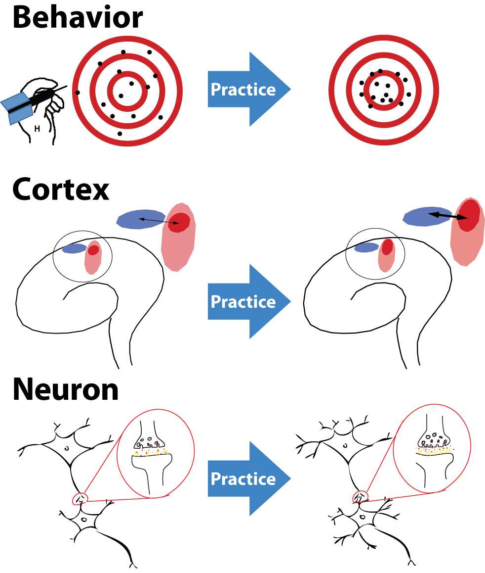
Neural plasticity and learning are fundamental adaptive processes that enable the brain to modify its structure and function in response to experience. Shown is a simplified schematic illustration of plastic changes induced by intensive practice of a specific skill at multiple organizational levels. Top (behavior): Repeated practice improves behavioral performance, illustrated here by increased accuracy and reduced variability when practicing a motor task such as throwing darts. Middle (cortex): At the cortical level, practice leads to a reorganization of functional representations, with task relevant neural populations becoming more strongly engaged and more precisely tuned. Bottom (neuron): At the cellular level, these changes are supported by synaptic and structural plasticity, including modifications of synaptic strength and local connectivity at individual neurons. Together, these coordinated changes across scales illustrate how learning emerges from local plastic mechanisms to produce stable improvements in behavior. Source: Wikimedia Commonsꜛ (license: CC BY 3.0).

Overview: Neuronal plasticity across scales

So, what are we talking about when we refer to neuronal plasticity? Broadly speaking, neuronal plasticity denotes the capacity of the nervous system to change both its functional properties and its underlying biological substrate (e.g., synaptic strengths, intrinsic excitability, structural connectivity) as a consequence of experience, ongoing activity, and environmental conditions (Bear et al., 2016ꜛ; Gerstner et al., 2014ꜛ). These changes may affect how neurons respond to inputs, how strongly they influence one another, and how information is represented and processed at the level of circuits and networks. For this reason, neuronal plasticity is widely regarded as the biological substrate of learning, memory formation, and behavioral adaptation (Dayan & Abbott, 2001ꜛ; Bear et al., 2016ꜛ).

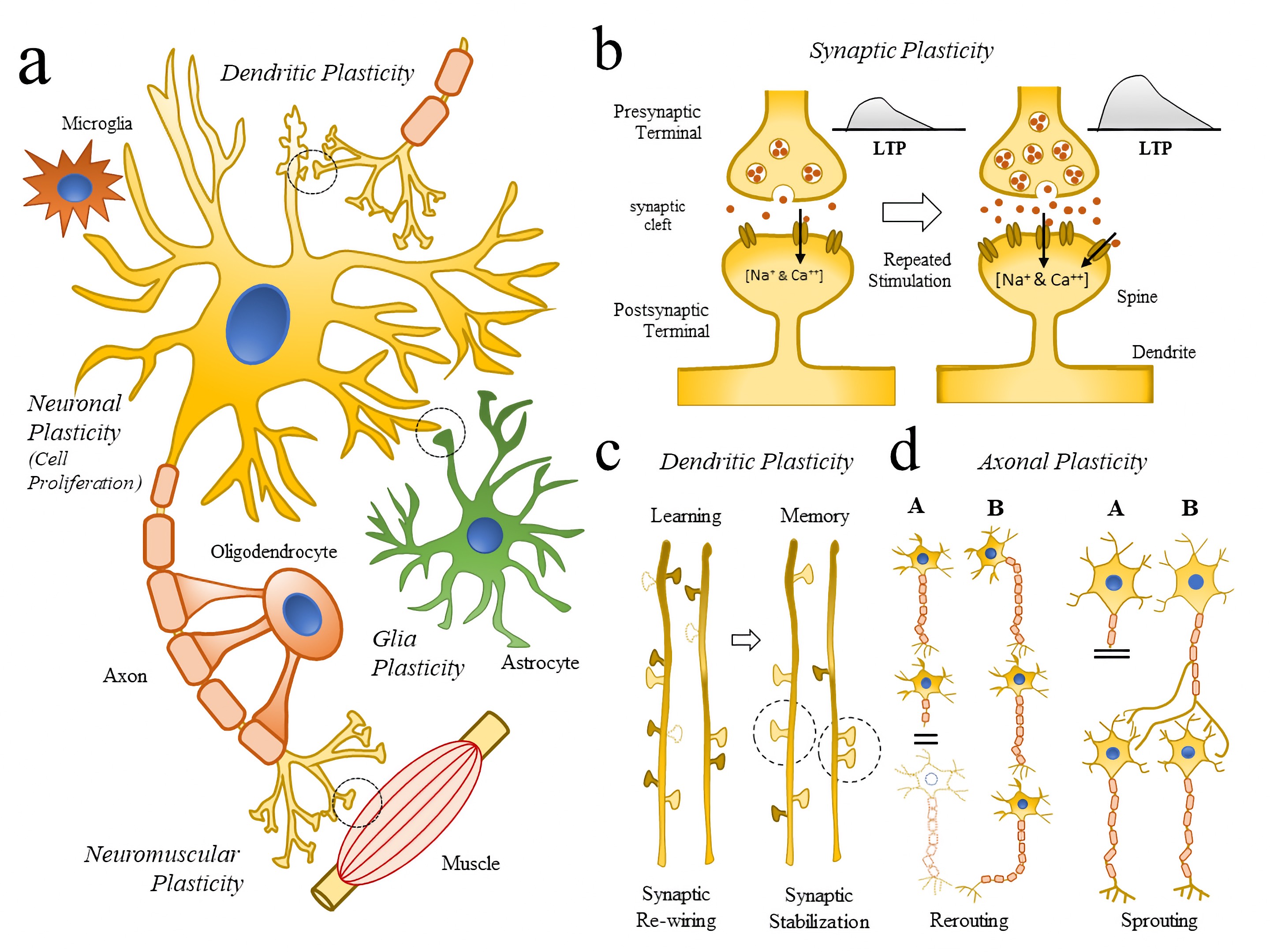Schematic illustration of neuronal plasticity across scales. (a) Schematic representation of key cellular elements (neuronal and glial cells) involved in the neuroplasticity (NP) process (Neuronal and Glia plasticity) as well as subcellular compartments (Synaptic, Dendritic, Axonal, Neuromuscular Plasticity). (b) Schematic diagram representing how repetitive synaptic stimulations repetitive LTPs are linked to molecular changes (Doted circle in (a)), and the generation of dendrite and spine remodeling. (c) Schematic illustration showing some of the changes in dendrite formations (dotted dendrite spines) following learning (synaptic re-wiring) and memory formation (synaptic stabilization). (d) Schematic illustration showing axonal mechanism of neuroplasticity and repair (rerouting and sprouting) following brain injury. Abbreviations: LTP, long-term potential. Source: Wikimediaꜛ (license: CC BY-SA 4.0; original figure from Gatto, 2020ꜛ).

Importantly, plasticity should not be understood as a single, uniform mechanism. Rather, it comprises a heterogeneous set of processes that operate on different spatial and temporal scales (Malenka & Bear, 2004ꜛ; Turrigiano & Nelson, 2004ꜛ). Some forms act locally and rapidly, such as activity dependent changes in synaptic efficacy, while others unfold over longer time scales and involve structural remodeling of neurons or the reorganization of entire cortical representations (Holtmaat & Svoboda, 2009ꜛ). Together, these processes allow neural systems to remain adaptable over short time scales while preserving stable function over the lifetime of an organism (Zenke et al., 2017ꜛ).

To make this more concrete, it is useful to distinguish several major forms of plasticity, which differ in the level at which they act, the mechanisms they involve, and the time scales on which they operate (Bear et al., 2016ꜛ):

synaptic plasticity
intrinsic plasticity
structural plasticity
plasticity of cortical maps

At the most fine grained level, synaptic plasticity refers to changes in the efficacy of individual synapses. Long term potentiation and long term depression are the canonical examples and have been studied extensively as cellular correlates of learning and memory (Bliss & Lomo, 1973ꜛ; Malenka & Bear, 2004ꜛ). Beyond these classical forms, spike timing dependent plasticity and its extensions relate synaptic change to the precise temporal structure of neural activity (Markram et al., 1997ꜛ; Bi & Poo, 1998ꜛ; Caporale & Dan, 2008ꜛ).

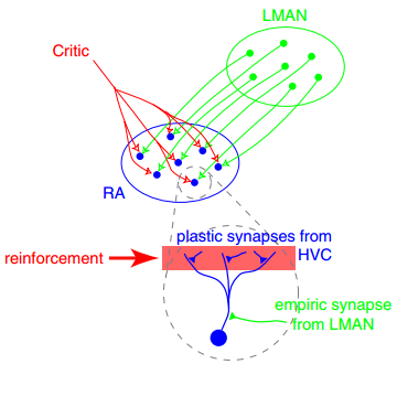
Example of synaptic plasticity. Shown is a synaptic plasticity rule for gradient estimation based on dynamic perturbations of synaptic conductances. Neurons in the exploratory circuit (LMAN) introduce stochastic perturbations to the activity of neurons in RA, a premotor motor area, via dedicated perturbation synapses. A critic evaluates behavioral performance and broadcasts a global reinforcement signal to plastic synapses, in particular the corticocortical projections from HVC (a premotor area) to RA (the motor area). Each synapse computes the product of its local perturbation and the global reinforcement signal and integrates this quantity over time to estimate the gradient of expected reward with respect to its synaptic weight. Synaptic weights are then adjusted in the direction of this estimated gradient, enabling reward-based optimization of motor output. Source: Wikimedia Commonsꜛ (license: CC BY 3.0).

Intrinsic plasticity captures changes in the excitability of individual neurons. By modifying ion channel expression, membrane time constants, or firing thresholds, neurons can adapt their input-output relationships without altering synaptic weights (Turrigiano, 2008ꜛ). These mechanisms regulate gain, responsiveness, and temporal filtering and thus shape how synaptic inputs are transformed into spikes (Buonomano & Maass, 2009ꜛ).

Structural plasticity describes morphological reorganization, such as the formation and elimination of dendritic spines, axonal boutons, and even larger scale dendritic and axonal remodeling (Yuste, 2010ꜛ; Holtmaat & Svoboda, 2009ꜛ). These changes alter the physical wiring diagram of the network and therefore its effective connectivity and representational capacity over longer time scales (Bernardinelli et al., 2014ꜛ).

In computational models, such as those we have explored in our previous post, structural plasticity is typically implemented at an abstract level, where the formation and elimination of synapses represents the functional outcome of underlying morphological processes rather than their detailed biophysical realization (Butz & van Ooyen, 2013ꜛ; Gerstner et al., 2014ꜛ).

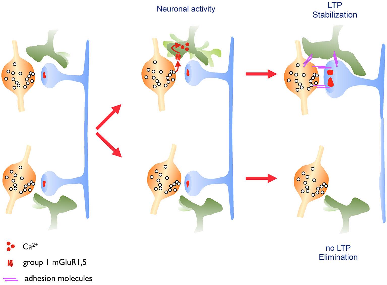Sketch illustrating astrocytic structural plasticity and synapse stabilization. The sketch illustrates how activity dependent remodeling of astrocytic processes contributes to the long term maintenance of activated synapses. Left: Excitatory synapses are dynamically contacted by highly motile astrocytic processes, reflecting ongoing structural plasticity in the tripartite synapse. Middle: Neurotransmitter release during neuronal activity activates metabotropic glutamate receptors on astrocytic processes, leading to intracellular calcium signaling and increased motility of astrocytic extensions. Right: Under learning related conditions that induce long term potentiation (upper synapse), enhanced astrocytic motility results in increased and persistent coverage of the synapse, promoting its stabilization. In contrast, synapses that are not potentiated (lower synapse) fail to recruit stable astrocytic contacts and are preferentially eliminated. Adhesion molecules are thought to contribute to this stabilization process. Source: Bernardinelli, Y., Nikonenko, I., Muller, D., Structural plasticity: mechanisms and contribution to developmental psychiatric disorders, Frontiers in Neuroanatomy, 2014, 8:123, doi 10.3389/fnana.2014.00123ꜛ (license: CC BY 4.0).

Finally, plasticity of cortical maps refers to the reorganization of large scale representations, for example after sensory deprivation, focal lesions, or prolonged training. Such reorganization reflects the coordinated outcome of synaptic, intrinsic, and structural plasticity operating across many neurons (Bear et al., 2016ꜛ; Gatto, 2020ꜛ).

In computational neuroscience, synaptic plasticity has traditionally taken center stage because it can be directly translated into mathematical learning rules (Dayan & Abbott, 2001ꜛ; Gerstner et al., 2014ꜛ). Correlation based rate models, including the classical Hebbian rule (Hebb, 1949ꜛ),

\[\Delta w_{ij} \propto \text{pre}_i \times \text{post}_j,\]

and its stabilized and extended variants such as Oja’s rule (Oja, 1982ꜛ)

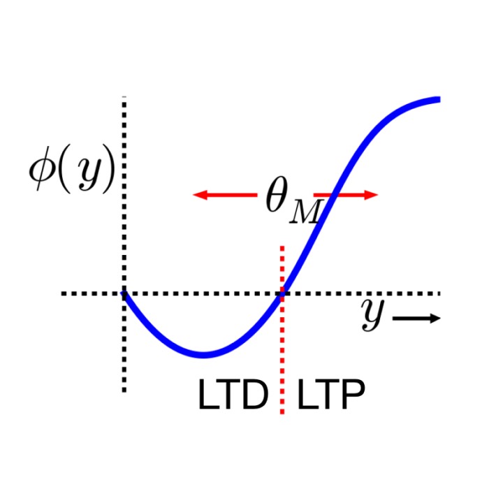
\[\Delta w_{ij} \propto \text{pre}_i \times \text{post}_j - \alpha \, \text{post}_j^2 \, w_{ij},\]

and the BCM framework (Bienenstock et al., 1982ꜛ; Shouval, 2007ꜛ)

\[\Delta w_{ij} \propto \text{pre}_i \times \text{post}_j \, (\text{post}_j - \theta_M),\]

describe how synaptic weights depend on averaged firing rates. Later, spike based formulations were introduced, most prominently spike timing dependent plasticity (STDP), which ties synaptic change to millisecond precise spike timing (Markram et al., 1997ꜛ; Morrison et al., 2008ꜛ). More recent developments, including triplet and higher order STDP models, three factor learning rules, and reward modulated plasticity, explicitly link synaptic mechanisms to learning at the behavioral and systems level (Pfister & Gerstner, 2006ꜛ; Fusi & Abbott, 2007ꜛ).

For this reason, synaptic plasticity remains the best studied and most formalized form of neuronal plasticity. At the same time, it must be understood as part of a broader plasticity landscape in which multiple mechanisms interact (Zenke et al., 2017ꜛ).

What is learning and how does it relate to plasticity?

Plasticity and learning are closely related but conceptually distinct notions. While plasticity refers to concrete biological mechanisms that change the properties of neurons and circuits, learning denotes the functional outcome of these changes at the level of behavior and internal representations (Bear et al., 2016ꜛ; Dayan & Abbott, 2001ꜛ). Clarifying this distinction is essential, especially when moving between biological description and computational modeling.

In neuroscience, learning is commonly defined as any persistent change in behavior or internal representations that arises from experience, training, or interaction with the environment (Hebb, 1949ꜛ; Bear et al., 2016ꜛ). These changes are functional rather than structural per se: They manifest as improved performance, the acquisition of new skills, the formation of memories, or the refinement of decisions and actions. Learning is therefore a system-level phenomenon, expressed in the dynamics of neural populations and their ability to generate stable, context-appropriate activity patterns (Buonomano & Maass, 2009ꜛ).

Left: Little child learns to take its first steps (Source: Nathan Dumlaoꜛ from Unspashꜛ, license: Unsplash Licenseꜛ). Right: A monkey mother teaches her baby how to climb (Source: Anirudh Chaudharyꜛ from Unspashꜛ, license: Unsplash Licenseꜛ). Learning is a fundamental adaptive process that enables organisms to acquire new skills and knowledge through experience, practice, and social interaction. In biological terms, learning is underpinned by various forms of neuronal plasticity that modify synaptic strengths, intrinsic excitability, and network connectivity. These plastic changes reshape neural dynamics, allowing the brain to form stable representations, improve performance, and adapt behaviorally to changing environments.

Crucially, learning should not be identified with any single plasticity mechanism. No individual synaptic modification, intrinsic adjustment, or structural change constitutes learning on its own (Malenka & Bear, 2004ꜛ; Turrigiano & Nelson, 2004ꜛ). Instead, learning emerges from the coordinated interaction of many plastic processes acting across different organizational levels. Through this coordination, neural networks adapt their dynamics such that certain patterns of activity become more reliable, more discriminable, or more easily reactivated (Fusi & Abbott, 2007ꜛ; Zenke et al., 2017ꜛ).

From this perspective, plasticity provides the mechanistic substrate of learning, while learning itself is the emergent reorganization of network function. Synaptic, intrinsic, and structural plasticity shape how neurons interact, how activity propagates through circuits, and which population states become stable or transient (Holtmaat & Svoboda, 2009ꜛ; Yuste, 2010ꜛ). The result is not merely a modified wiring diagram or altered excitability, but a transformed dynamical system capable of representing and using information in new ways (Gerstner et al., 2014ꜛ).

This distinction becomes particularly important in computational neuroscience. Models typically implement learning as parameter adaptation, for example changes in synaptic weights, thresholds, or connectivity (Dayan & Abbott, 2001ꜛ; Gerstner et al., 2014ꜛ). These parameter changes correspond to specific forms of biological plasticity. Learning, however, is assessed at a different level: By changes in network dynamics, attractor structure, representational geometry, or behavioral output (Buonomano & Maass, 2009ꜛ; Gao et al., 2017ꜛ). In this sense, plasticity is local and mechanistic, whereas learning is global and functional.

Learning as dynamical reorganization of neural systems

From a computational perspective, learning is most naturally described within the framework of dynamical systems (Dayan & Abbott, 2001ꜛ; Gerstner et al., 2014ꜛ). Neural networks are not static input–output mappings, but evolving systems whose internal state changes continuously in time as a function of ongoing activity, external inputs, and slowly adapting parameters. Learning corresponds to persistent, experience dependent modifications of this dynamical system (Buonomano & Maass, 2009ꜛ).

Formally, the internal state of a network evolves according to a set of coupled differential equations

\[\dot{x}(t) = f\big(x(t), u(t); W, \theta, \ldots \big),\]

where $x(t) \in \mathbb{R}^N$ denotes the vector of neural states, such as firing rates or membrane potentials of $N$ neurons, $u(t)$ represents external inputs, $W$ the synaptic weight matrix, and $\theta$ other parameters including thresholds, gains, or time constants. Network outputs are given by a readout mapping

\[y(t) = g\big(x(t)\big),\]

which may correspond to motor commands, decisions, or downstream neural signals. The functions $f$ and $g$ jointly define the intrinsic dynamics and the observable behavior of the network (Gerstner et al., 2014ꜛ).

Within this formalism, learning can be defined as any persistent, experience dependent change in the network dynamics $f$ and/or in the parameter set $\Theta = {W, \theta, \ldots}$ that alters the mapping from inputs $u(t)$ to internal states $x(t)$ and outputs $y(t)$ in a functionally beneficial way. Such benefits may include improved robustness of representations, enhanced recall, better generalization, or more reliable goal directed behavior (Fusi & Abbott, 2007ꜛ). Plasticity provides the mechanistic substrate for these changes, while learning is the emergent consequence at the level of network dynamics.

A key structural feature of biological learning systems is the separation of time scales. Neural activity typically evolves on fast time scales, while parameters adapt much more slowly (Zenke et al., 2017ꜛ). This can be expressed explicitly as a coupled slow–fast system

\[\begin{aligned} \dot{x} &= f(x, u; \Theta), \\ \dot{\Theta} &= \varepsilon \, \mathcal{L}(x, u, y, r; \Theta), \end{aligned}\]

with $0 < \varepsilon \ll 1$. Here, $\mathcal{L}$ denotes a learning rule that may depend on local pre- and postsynaptic activity, global modulatory signals such as reinforcement or error feedback $r$, and additional contextual variables(Gerstner et al., 2014ꜛ; Zenke et al., 2017ꜛ). On short time scales, the parameters can be treated as quasi-static, while on longer time scales their gradual evolution reshapes the dynamical landscape of the system.

A useful geometric interpretation arises by viewing the activity of a population of $N$ neurons at any moment in time as a point $x \in \mathbb{R}^N$ in neural state space. As time evolves, network activity traces out trajectories through this space (Buonomano & Maass, 2009ꜛ; Gao et al., 2017ꜛ). Learning reshapes these trajectories by modifying the underlying vector field defined by $f$. In many cases, plasticity causes trajectories to concentrate onto low dimensional manifolds embedded in the high dimensional state space (Gao et al., 2017ꜛ; Song et al., 2023ꜛ). These manifolds encode task relevant variables, categories, or internal states, while suppressing variability along irrelevant dimensions.

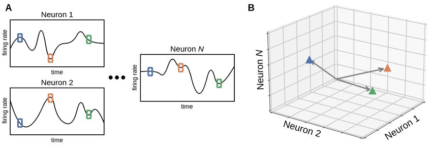Neural state space representation of population activity. (A) The activity of individual neurons is shown as time dependent signals, for example firing rates or other measures of neural activation. Colored markers indicate the joint activity pattern across all recorded neurons at specific time points. (B) At each time point, the collective activity of a population of $N$ neurons defines a single point in an $N$ dimensional neural state space. As time evolves, neural dynamics correspond to trajectories through this space, providing a geometric description of population activity that underlies representation, computation, and learning. Source: Ji, X., Elmoznino, E., Deane, G., Constant, A., Dumas, G., Lajoie, G., Bengio, Y., Sources of richness and ineffability for phenomenally conscious states, 2023, preprint, arXiv, doi: 10.48550/arXiv.2302.06403ꜛ; Figure available via ResearchGateꜛ (license: CC BY-SA 4.0)

From this viewpoint, learning corresponds to a geometric reorganization of population activity. Distances between trajectories representing different stimuli or decisions may increase, improving separability, while variability within behaviorally equivalent states may contract, enhancing robustness and generalization (Gao et al., 2017ꜛ).

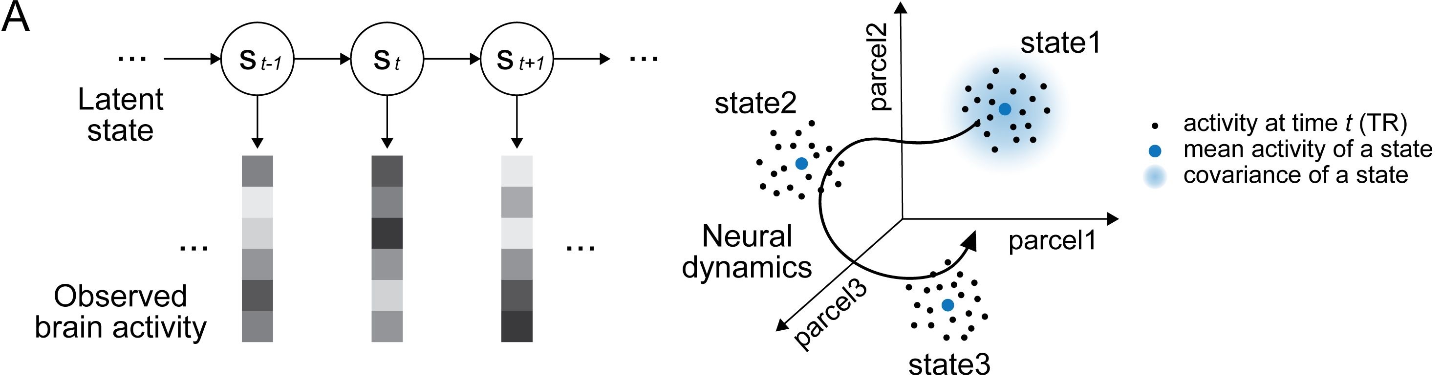Latent state space of large-scale neural dynamics. The figure illustrates how high-dimensional neural activity can be described in terms of low-dimensional latent states that capture the dominant network dynamics. Shown on the left is a schematic illustration of hidden Markov model (HMM) inference applied to large-scale brain activity. Here, from observed multivariate fMRI time series, the model infers a sequence of discrete latent states that summarize recurrent patterns of population activity. On the right, neural activity can be visualized as trajectories through a high-dimensional state space, here defined by activity across multiple cortical parcels. The HMM identifies latent clusters within this space, where each state is characterized by its mean activity pattern and covariance structure. Transitions between states reflect the underlying network dynamics and provide a compact description of how neural activity evolves over time. Source: Figure 1A from Song, H., Shim, W. M., Rosenberg, M. D., Large-scale neural dynamics in a shared low-dimensional state space reflect cognitive and attentional dynamics, eLife, 2023, 12:e85487, doi: 10.7554/eLife.85487ꜛ (license: CC BY 4.0; modified (cropped)); adapted from Cornblath et al., 2020ꜛ.

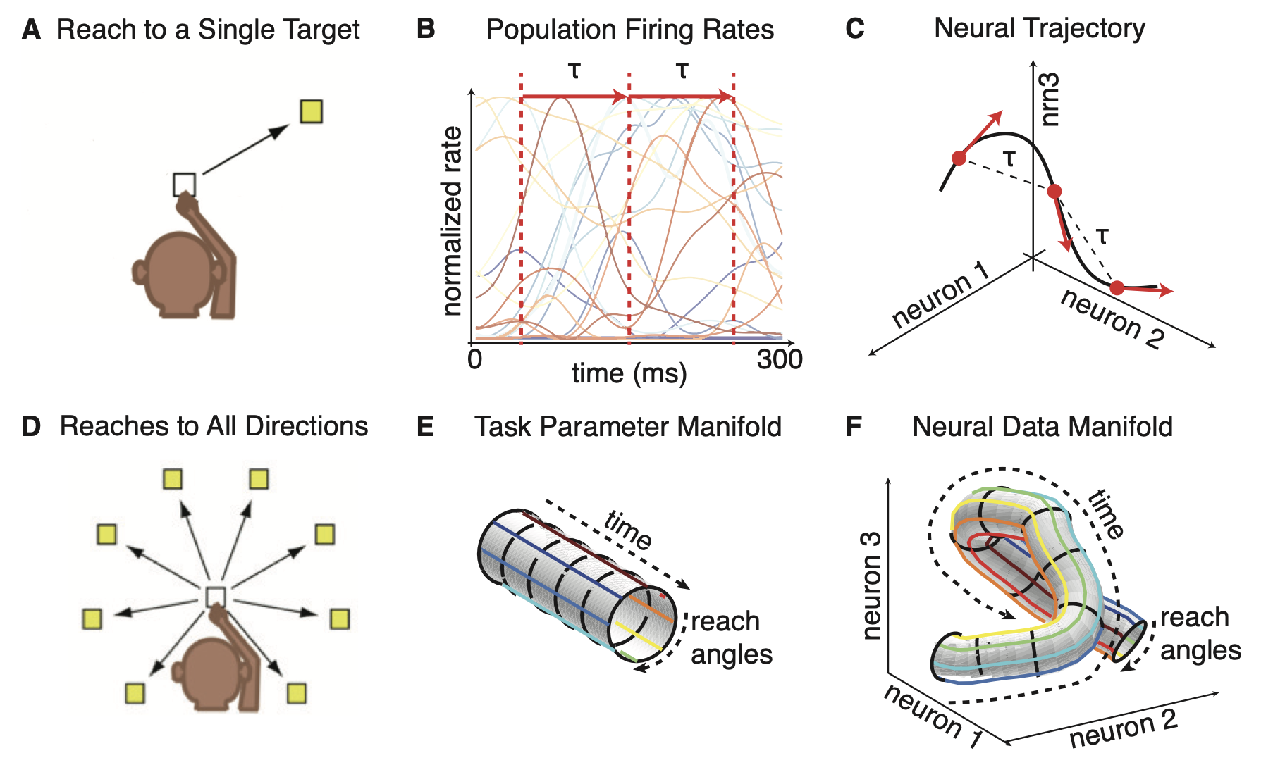Neural population dynamics as an embedding of task structure into neural state space. (A) Behavioral paradigm illustrating a reaching movement to a single target. The monkey initiates a movement from a fixed starting position and reaches toward a specified goal. In this simple condition, the task is fully parameterized by time $t$ along the movement trajectory. (B) Trial-averaged population firing rates of many simultaneously recorded neurons during the reach. Each trace represents the activity of one neuron as a function of time, illustrating how complex, heterogeneous single-neuron responses unfold during a structured behavior. (C) The same population activity represented as a trajectory in neural state space. At each time point, the joint activity of all recorded neurons defines a single point in a high-dimensional space, with neural dynamics corresponding to a continuous trajectory through this space. Temporal evolution of behavior is thus mapped onto a geometric path in population activity space. (D) Extension of the task to reaching movements in multiple directions. In this case, behavior is no longer described by time alone but by two task variables: Time within the movement and reach angle. (E) The resulting task manifold, here shown schematically as a low-dimensional cylinder parameterized by time and reach direction. Each point on this manifold corresponds to a specific behavioral state of the task. (F) The neural data manifold obtained from population activity. Neural trajectories corresponding to different reach directions form a smooth, structured surface in neural state space, demonstrating that population activity provides a continuous embedding of the low-dimensional task manifold into a high-dimensional neural space. This illustrates how neural manifolds capture both task structure and dynamics, and how learning and experience shape the geometry of population activity. Source: Figure 3 from Gao, P., Trautmann, E., Yu, B., Santhanam, G., Ryu, S., Shenoy, K., Ganguli, S., A theory of multineuronal dimensionality, dynamics and measurement, 2017, bioRxiv 214262, doi: 10.1101/214262ꜛ (license: CC BY 4.0).

Learned information often manifests as the stability of particular regions of state space, which motivates an attractor based interpretation (Hopfield, 1982ꜛ; Gerstner et al., 2014ꜛ). An attractor $\mathcal{A}$ is a set toward which trajectories converge for a range of initial conditions. Local stability of a fixed point attractor $x^*$, for example, can be characterized by the eigenvalues of the Jacobian

\[J = \left. \frac{\partial f}{\partial x} \right|_{x = x^\ast},\]

with stability requiring that all eigenvalues have negative real parts (Strogatz, 1998; Gerstner et al., 2014ꜛ). Plasticity modifies $f$ and therefore alters both the location and stability of attractors. New attractors may emerge, existing attractors may shift or merge, and others may lose stability (Curto & Morrison, 2023ꜛ).

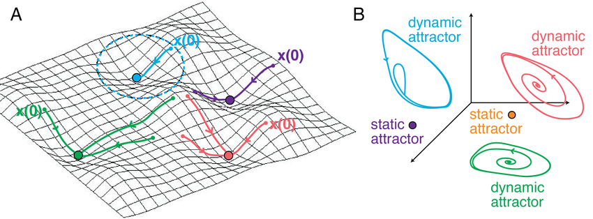(A) In recurrent networks with symmetric interactions, such as Hopfield type networks, neural activity evolves toward stable fixed point attractors. Independent of initial conditions, trajectories converge into basins of attraction that correspond to stored or learned network states. The illustrated trajectories show how different initial states relax into distinct stable fixed points. (B) In networks with asymmetric connectivity, fixed point attractors can coexist with dynamic attractors, such as limit cycles or more complex recurrent trajectories. These dynamic attractors support sustained, time dependent activity patterns and illustrate how learning can give rise not only to static memory states but also to structured temporal dynamics. Source: Curto & Morrison, Graph rules for recurrent neural network dynamics: extended version, 2023, preprint, arXiv, doi: 10.48550/arXiv.2301.12638ꜛ, ResearchGateꜛ (license: CC BY-SA 4.0)

Different classes of attractors support different computational functions. Fixed point attractors underlie associative memory and pattern completion (Hopfield, 1982ꜛ), continuous attractors represent continuous variables such as position or orientation, and dynamic attractors including limit cycles or more complex trajectories enable temporal and sequential computations (Buonomano & Maass, 2009ꜛ). Plasticity mechanisms such as Hebbian learning (Hebb, 1949ꜛ), BCM type rules (Bienenstock et al., 1982ꜛ), and spike timing dependent plasticity (STDP) (Bi & Poo, 1998ꜛ; Caporale & Dan, 2008ꜛ) selectively stabilize patterns of coactivity, thereby shaping the attractor landscape of the network.

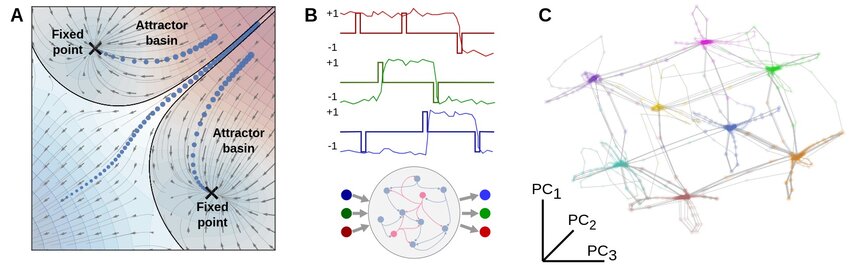Attractor dynamics and memory representations in neural networks. (A) Schematic illustration of attractors in a low dimensional neural state space. Once network activity enters the basin of attraction of a fixed point, trajectories converge toward that attractor and remain stable unless perturbed by external input or intrinsic noise. (B) Example dynamics from a recurrent neural network (RNN) trained to perform a working memory task, where the network must maintain and update binary information across multiple input channels. Task relevant variables are encoded in stable patterns of population activity. (C) In the trained network, fixed point attractors emerge as solutions to the task. Each attractor corresponds to a distinct memory state, here representing one of the possible input configurations. Neural trajectories evolve between these attractors as inputs change. For visualization, the high dimensional state space of the network is projected onto its leading principal components. Source: Ji, X., Elmoznino, E., Deane, G., Constant, A., Dumas, G., Lajoie, G., Bengio, Y., Sources of richness and ineffability for phenomenally conscious states, 2023, preprint, arXiv, doi: 10.48550/arXiv.2302.06403ꜛ; Figure available via ResearchGateꜛ (license: CC BY-SA 4.0)

Learning can thus be understood as a reorganization of the network’s attractor structure. Experiences become embedded as stable or metastable dynamical regimes that can be reliably reactivated by partial input or contextual cues (Fusi & Abbott, 2007ꜛ). At the same time, learning systems must resolve the stability plasticity dilemma. Plasticity must be sufficiently strong to allow adaptation, yet sufficiently regulated to prevent catastrophic interference with previously acquired knowledge (Zenke et al., 2017ꜛ). Homeostatic mechanisms, normalization, and metaplasticity constrain parameter drift and help maintain global dynamical stability (Turrigiano & Nelson, 2004ꜛ; Turrigiano, 2008ꜛ).

In summary, learning in neural systems is best understood not as a single mechanism or parameter change, but as the slow, experience driven reconfiguration of a high dimensional dynamical system. Plasticity acts locally and mechanistically at synapses and neurons, while learning emerges globally as a transformation of neural dynamics, representational geometry, and attractor structure.

Learning paradigms and signals

The form of plasticity depends strongly on the learning context. Three major paradigms can be distinguished: unsupervised, reinforcement based, and error driven learning.

In unsupervised settings, synaptic changes are driven solely by correlations within the neural activity itself. Classical Hebbian (Hebb, 1949ꜛ), covariance, Oja (Oja, 1982ꜛ), and BCM rules (Bienenstock et al., 1982ꜛ; Shouval, 2007ꜛ) can be understood as local estimates of input statistics. In rate-based form, these rules typically depend on low-order moments of pre- and postsynaptic activity and lead to feature extraction, receptive field formation, and dimensionality reduction (Dayan & Abbott, 2001ꜛ). From a dynamical perspective, such rules reshape the flow field of the network so that frequently co-active patterns become more stable or more strongly amplified (Buonomano & Maass, 2009ꜛ).

Reinforcement-based learning introduces an additional global signal that evaluates the outcome of neural activity rather than its detailed structure. Because rewards or punishments are often delayed relative to the neural events that caused them, synaptic updates rely on eligibility traces that temporally bridge this gap (Gerstner et al., 2014ꜛ; Zenke et al., 2017ꜛ). A generic formulation is

\[\dot e_{ij}(t) = \phi(\text{pre}_i(t), \text{post}_j(t)) - \frac{e_{ij}(t)}{\tau_e},\]

where $e_{ij}$ is a synapse-specific eligibility trace and $\tau_e$ its decay time constant. Weight changes then take the form

\[\dot w_{ij}(t) = \eta \, e_{ij}(t) \, r(t),\]

with $r(t)$ denoting a global reinforcement or modulatory signal, often associated with dopaminergic input (Gerstner et al., 2014ꜛ). In this view, reinforcement learning is not a distinct plasticity mechanism, but a particular factorization of the learning rule into local activity-dependent terms and a global scalar signal.

Error-driven learning represents a special case in which explicit teaching or error signals are available. This is well established in cerebellar circuits, where climbing fiber input conveys performance errors (Dayan & Abbott, 2001ꜛ). In cortical systems, however, direct error signals are rare, and many phenomena that appear error-driven at the behavioral level can be interpreted as reinforcement-like modulation of otherwise local plasticity rules (Fusi & Abbott, 2007ꜛ; Zenke et al., 2017ꜛ). Across paradigms, the common structure is that learning rules estimate how changes in synaptic parameters influence future network dynamics and behavioral outcomes.

Time and spatial scales

Plasticity and learning unfold across a hierarchy of time and spatial scales, and this hierarchy is essential for stable adaptation (Fusi & Abbott, 2007ꜛ; Zenke et al., 2017ꜛ). At the fastest level, neural states $x(t)$ evolve on millisecond time scales according to the intrinsic dynamics of neurons and synapses. Plastic changes act on slower variables, introducing a separation of time scales that can be expressed schematically as

\[\dot x = f(x, u; W), \quad \dot W = \epsilon \, \mathcal{L}(x, \ldots),\]

with $\epsilon \ll 1$.

On short time scales ranging from milliseconds to minutes, mechanisms such as short-term synaptic plasticity, spike-timing–dependent eligibility traces, and early phases of long-term potentiation and depression transiently tag relevant patterns of activity (Bi & Poo, 1998ꜛ; Pfister & Gerstner, 2006ꜛ; Caporale & Dan, 2008ꜛ). These mechanisms bias subsequent plasticity without permanently altering network structure.

On intermediate time scales of hours to days, late-phase LTP and LTD, spine stabilization, and local circuit reorganization consolidate these transient changes (Bliss & Lomo, 1973ꜛ; Malenka & Bear, 2004ꜛ; Holtmaat & Svoboda, 2009ꜛ). At this level, learning becomes robust to noise and perturbations, and newly formed attractors or manifolds persist beyond the immediate learning episode (Fusi & Abbott, 2007ꜛ).

On long time scales of days to years, large-scale cortical reorganization, systems consolidation from hippocampus to neocortex, and the automatization of skills take place (Turrigiano & Nelson, 2004ꜛ; Turrigiano, 2008ꜛ). These slow processes effectively reshape the parameter landscape of the network, constraining future learning and enabling lifelong accumulation of knowledge.

Importantly, learning alternates between online phases during active behavior and offline phases during sleep or rest. Offline replay and reactivation can be interpreted as additional trajectories through neural state space that reinforce or refine previously formed attractors while reducing interference between memories (Buonomano & Maass, 2009ꜛ; Zenke et al., 2017ꜛ).

Rates versus spike timing

Whether learning is best described in terms of firing rates or precise spike timing depends on the temporal resolution required to capture the relevant dynamics (Dayan & Abbott, 2001ꜛ; Gerstner et al., 2014ꜛ). Spike-based models explicitly represent action potentials and can express learning rules that depend on millisecond-scale timing differences, as in STDP (Markram et al., 1997ꜛ; Bi & Poo, 1998ꜛ; Caporale & Dan, 2008ꜛ). These mechanisms are essential for tasks involving temporal sequences, causality, or fine sensory discrimination (Buonomano & Maass, 2009ꜛ).

Rate-based models, in contrast, describe neural activity as temporally averaged variables (Dayan & Abbott, 2001ꜛ). They are often sufficient for capturing the stabilization of attractors, working memory, decision-making processes, and other phenomena that depend primarily on slower collective dynamics (Hopfield, 1982ꜛ; Buonomano & Maass, 2009ꜛ). Mathematically, rate models can be viewed as coarse-grained descriptions of underlying spiking dynamics, obtained by averaging over fast fluctuations (Gerstner et al., 2014ꜛ).

Bridging models such as triplet STDP demonstrate how spike-based rules reduce, under temporal averaging, to rate-based learning rules like BCM (Pfister & Gerstner, 2006ꜛ; Shouval, 2007ꜛ). In this sense, rate and spike formulations do not represent competing theories, but different projections of the same underlying dynamical system onto different time scales (Zenke et al., 2017ꜛ). The appropriate description is determined by the question being asked rather than by biological realism alone.

Practical implications for experiments and modeling

Viewing learning as a dynamical reorganization of neural systems has direct implications for both experimental design and computational modeling (Buonomano & Maass, 2009ꜛ; Gerstner et al., 2014ꜛ). At the behavioral level, learning manifests as increased accuracy, improved robustness to noise, and more reliable reward maximization. These behavioral changes correspond to increased stability and separability of neural representations (Fusi & Abbott, 2007ꜛ).

At the neurophysiological level, learning is reflected in changes to population activity rather than isolated neurons. Observable signatures include reduced dimensionality of task-relevant activity, reshaped manifolds in neural state space, and the emergence or stabilization of attractors (Gao et al., 2017ꜛ; Song et al., 2023ꜛ). These effects are often invisible at the level of single-neuron tuning curves but become apparent when analyzing population trajectories.

At the anatomical and biophysical level, learning leaves persistent traces in spine stability, receptor composition, intrinsic excitability, and connectivity patterns (Holtmaat & Svoboda, 2009ꜛ; Yuste, 2010ꜛ). These changes constrain future dynamics and bias the system toward previously learned solutions.

From a theoretical perspective, learning corresponds to changes in the qualitative structure of the dynamical system. Fixed points may be created or displaced, eigenvalue spectra of the linearized dynamics may shift, and basins of attraction may expand or contract (Gerstner et al., 2014ꜛ; Curto & Morrison, 2023ꜛ). Improved generalization and robustness can often be traced back to increased margins between representations in state space and to the stabilization of task-relevant directions of activity (Fusi & Abbott, 2007ꜛ; Gao et al., 2017ꜛ).

A compact formal summary

Bringing these ideas together, we can condense them into a minimal formal description that captures the essential structure of learning in neural systems.

Network dynamics are described by

\[\dot{x} = f(x, u; \Theta),\]

where $x$ denotes the network state, $u$ external inputs, and $\Theta$ the set of parameters governing the dynamics.

Learning corresponds to experience dependent changes of these parameters according to

\[\dot{\Theta} = \mathcal{L}(x, u, y, r; \Theta),\]

with $\mathcal{L}$ denoting a learning rule that may depend on local activity, global modulatory signals, or behavioral feedback.

Through this coupled evolution, learning reshapes the geometry of neural state space and the attractor structure of the dynamics, enabling stable representations, flexible computation, and adaptive behavior under biological constraints.

Concluding perspective

What we can take away from this discussion is that neuronal plasticity and learning describe different levels of the same adaptive process. Plasticity refers to the biological mechanisms by which neural systems change, while learning denotes the functional outcome of these changes at the level of network dynamics, representations, and behavior. Learning does not reside in individual synapses or neurons, but emerges from the coordinated interaction of multiple plastic processes acting across spatial and temporal scales.

From a computational viewpoint, this distinction is crucial. Local plasticity mechanisms modify parameters or connectivity, whereas learning is expressed globally as a reorganization of neural state space and attractor structure. Changes in synaptic strength, intrinsic excitability, or network topology reshape the effective dynamics, giving rise to stable yet flexible patterns of population activity.

I believe, that this dynamical perspective provides a unifying framework for diverse modeling approaches in computational neuroscience. Rate based and spike based descriptions, different learning paradigms, and geometric or attractor based interpretations capture complementary aspects of how adaptive neural systems operate. Together, they emphasize that learning is best understood as a constrained, multiscale reconfiguration of network dynamics rather than as the outcome of any single plasticity rule.

As stated at the beginning of this post, the view presented here reflects my current understanding of the topic. It is intended as a conceptual reference point rather than a definitive account. As always, I welcome feedback, corrections, and suggestions for improvement in the comments below. Any new insights I gain will be incorporated into future updates of this post.

References and further reading

Marc F. Bear, Barry W. Connors, and Michael A. Paradiso, Neuroscience: Exploring the Brain, 2016, 4th edition, Wolters Kluwer, ISBN: 978-0-7817-7817-6ꜛ
Bernardinelli, Y., Nikonenko, I., Muller, D., Structural plasticity: mechanisms and contribution to developmental psychiatric disorders, 2014, Frontiers in Neuroanatomy, 8:123, doi 10.3389/fnana.2014.00123ꜛ
G. Bi, & M. Poo, Synaptic modifications in cultured hippocampal neurons: dependence on spike timing, synaptic strength, and postsynaptic cell type, 1998, Journal of neuroscience, doi: 10.1523/JNEUROSCI.18-24-10464.1998ꜛ
E. L. Bienenstock, L. N. Cooper, P. W. Munro, Theory for the development of neuron selectivity: orientation specificity and binocular interaction in visual cortex, 1982, Journal of Neuroscience, doi: 10.1523/JNEUROSCI.02-01-00032.1982ꜛ
Bliss TV, Lomo T. Long-lasting potentiation of synaptic transmission in the dentate area of the anaesthetized rabbit following stimulation of the perforant path, 1973, J Physiol., 232(2):331-56. doi: 10.1113/jphysiol.1973.sp010273ꜛ
Buonomano, Dean V., Maass, Wolfgang, State-dependent computations: spatiotemporal processing in cortical networks, Nature Reviews Neuroscience, 2009, 10(2), 113–125, doi: 10.1038/nrn2558ꜛ
Markus Butz, Arjen van Ooyen, A Simple Rule for Dendritic Spine and Axonal Bouton Formation Can Account for Cortical Reorganization after Focal Retinal Lesions, 2013, PLoS Computational Biology, Vol. 9, Issue 10, pages e1003259, doi: 10.1371/journal.pcbi.1003259
Natalia Caporale, & Yang Dan, Spike timing-dependent plasticity: a Hebbian learning rule, 2008, Annu Rev Neurosci, Vol. 31, pages 25-46, doi: 10.1146/annurev.neuro.31.060407.125639ꜛ
Carina Curto, Katherine Morrison, Graph rules for recurrent neural network dynamics: extended version, 2023, preprint, arXiv, doi: 10.48550/arXiv.2301.12638ꜛ
P. Dayan, I. F. Abbott, Theoretical Neuroscience: Computational and Mathematical Modeling of Neural Systems, 2001, MIT Press, ISBN: 0-262-04199-5ꜛ
Feldman, Daniel E., The spike-timing dependence of plasticity, 2012, Neuron;75(4):556-71. doi: 10.1016/j.neuron.2012.08.001ꜛ
Fusi, S., Abbott, L., Limits on the memory storage capacity of bounded synapses, 2007, Nat Neurosci 10, 485–493, doi: 10.1038/nn1859ꜛ
Rodolfo Gabriel Gatto, Molecular and microstructural biomarkers of neuroplasticity in neurodegenerative disorders through preclinical and diffusion magnetic resonance imaging studies, 2020, J. Integr. Neurosci., 19(3), 571–592. doi: 10.31083/j.jin.2020.03.165ꜛ
Gao, P., Trautmann, E., Yu, B., Santhanam, G., Ryu, S., Shenoy, K., Ganguli, S., A theory of multineuronal dimensionality, dynamics and measurement, 2017, bioRxiv 214262, doi: 10.1101/214262ꜛ
Wulfram Gerstner, Werner M. Kistler, Richard Naud, and Liam Paninski, Neuronal Dynamics: From Single Neurons to Networks and Models of Cognition, 2014, Cambridge University Press, ISBN: 978-1-107-06083-8, free online versionꜛ
Donald O. Hebb, The Organization of Behavior, 1949, Wiley: New York, doi: 10.1016/s0361-9230(99)00182-3ꜛ
Holtmaat, A., Svoboda, K., Experience-dependent structural synaptic plasticity in the mammalian brain, 2009, Nat Rev Neurosci 10, 647–658, doi: 10.1038/nrn2699ꜛ
Hopfield, John J., Neural networks and physical systems with emergent collective computational abilities, 1982, Proc Natl Acad Sci U S A, 79(8), 2554-2558. doi: 10.1073/pnas.79.8.2554
Ji, X., Elmoznino, E., Deane, G., Constant, A., Dumas, G., Lajoie, G., Bengio, Y., Sources of richness and ineffability for phenomenally conscious states, 2023, preprint, arXiv, doi: 10.48550/arXiv.2302.06403ꜛ
Malenka, Robert C., Bear, Mark F., LTP and LTD: An embarrassment of riches, 2004, Neuron, Vol. 44, Issue 1, pages 5-21, doi: 10.1016/j.neuron.2004.09.012ꜛ
H. Markram, J. Lübke, M. Frotscher, B. Sakmann, Regulation of Synaptic Efficacy by Coincidence of Postsynaptic APs and EPSPs, 1997, Science, Vol. 275, Issue 5297, pages 213-215, doi: 10.1126/science.275.5297.213ꜛ
Morrison, A, Diesmann, M, & Gerstner, W, Phenomenological models of synaptic plasticity based on spike timing, 2008, Biol Cybern, 98(6), 459-478. doi: 10.1007/s00422-008-0233-1ꜛ
E Oja, Simplified [neuron model as a principal component analyzer, 1982, Journal of mathematical biology, doi: 10.1007/BF00275687ꜛ
J. P. Pfister & Wulfram Gerstner, Triplets of spikes in a model of spike timing-dependent plasticity, 2006, Journal of [Neuroscience, doi: 10.1523/JNEUROSCI.1425-06.2006ꜛ
Pozo, Karen, Goda, Yukiko, Unraveling mechanisms of homeostatic synaptic plasticity, 2010, Neuron; 66(3):337-51. doi: 10.1016/j.neuron.2010.04.028ꜛ
Rumelhart, David E., McClelland, James L., PDP Research Group, Parallel Distributed Processing: Explorations in the Microstructure of Cognition, Volume 1, 1986, MIT Press, ISBN: 978-0262680530.
Harel Z. Shouval, Models of synaptic plasticity, 2007, Scholarpedia, 2(7):1605, doi: 10.4249/scholarpedia.1605ꜛ
Song, H., Shim, W. M., Rosenberg, M. D., Large-scale neural dynamics in a shared low-dimensional state space reflect cognitive and attentional dynamics, eLife, 2023, 12:e85487, doi: 10.7554/eLife.85487ꜛ
Steven H. Strogatz, Nonlinear Dynamics and Chaos. With Student Solutions Manual: With Applications to Physics, Biology, Chemistry, and Engineering, 1998, Book, CRC Press, ISBN: 0429680155
Turrigiano, Gina G., The self-tuning neuron: synaptic scaling of excitatory synapses, 2008, Cell; 135(3):422-35. doi: 10.1016/j.cell.2008.10.008ꜛ
Turrigiano, Gina G., Nelson, Sacha B., Homeostatic plasticity in the developing nervous system, 2004, Nature Reviews Neuroscience, 5(2), 97–107, doi: 10.1038/nrn1327ꜛ
Yuste, Rafael, Dendritic Spines, 2010, MIT Press, ISBN: 978-0262013505ꜛ
Zenke, F, Gerstner, W, & Ganguli, S, The temporal paradox of Hebbian learning and homeostatic plasticity (2017), Curr Opin Neurobiol, 43, 166-176. doi: 10.1016/j.conb.2017.03.015