Single-particle description of plasmas: Equation of motion, gyration, and ExB drift

June 6, 2020 January 9, 2026 21 minute read see also comments

As a first step toward understanding plasma dynamics, it is instructive to study the motion of a single charged particle, such as an electron or an ion, in prescribed electric and magnetic fields. In this approach, the electromagnetic fields are treated as externally given, and the fields generated by the particle itself and by other plasma particles are neglected. In other words, collective effects are deliberately ignored.

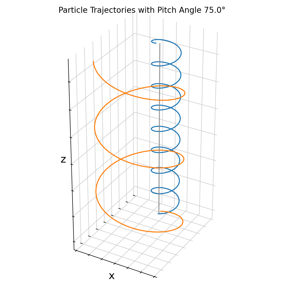
$Numerical simulation of charged-particles in a uniform magnetic field $\mathbf{B}$.$
Numerical simulation of charged-particles in a uniform magnetic field $\mathbf{B}$. The particles gyrate around magnetic field lines. Here, an electron (blue) and a positively charged ion (orange) are shown for a pitch angle of 75°.

This single-particle description is justified under several common conditions. It applies when the plasma is sufficiently dilute, when a chemical subpopulation with low number density is considered, such as doubly ionized helium in a hydrogen plasma, or when an energetic subpopulation with small phase-space density is studied, such as keV ions embedded in a thermal plasma with much lower characteristic energies. In these situations, the influence of the test particles on the global plasma fields is negligible, and their dynamics can be treated independently.

Equation of motion in electromagnetic fields

In the single-particle picture, the forces acting on a charged particle are the electric Coulomb force and the magnetic Lorentz force,

\[\begin{align} \mathbf{F}_C = q \mathbf{E}, \quad \mathbf{F}_L = q (\mathbf{v} \times \mathbf{B}), \end{align}\]

where $q$ is the particle charge, $\mathbf{v}$ its velocity, and $\mathbf{E}$ and $\mathbf{B}$ the electric and magnetic fields.

Applying Newton’s second law yields the equation of motion for a charged particle in electromagnetic fields,

\[\begin{align} m \, d_t \mathbf{v} = q \left( \mathbf{E} + \mathbf{v} \times \mathbf{B} \right), \end{align}\]

with $m$ the particle mass and $\mathbf{v} = d_t \mathbf{x}$ the time derivative of the particle position. This equation forms the basis of the single-particle description of plasmas.

Energy conservation and the role of the magnetic field

A key property of the Lorentz force is that the magnetic contribution is always perpendicular to the particle velocity. Taking the scalar product of the equation of motion with $\mathbf{v}$ and assuming $\mathbf{E} = 0$ yields

\[\begin{align} m \, \mathbf{v} \cdot d_t \mathbf{v} = q \, \mathbf{v} \cdot (\mathbf{v} \times \mathbf{B}) = 0. \end{align}\]

This implies

\[\begin{align} d_t \left( \frac{1}{2} m v^2 \right) = 0, \end{align}\]

so the kinetic energy of the particle remains constant. A static magnetic field performs no work on charged particles. It can change the direction of the velocity, but not its magnitude. This property is fundamental for understanding gyration and guiding-center motion.

Motion in a uniform magnetic field

To make this explicit, consider a homogeneous magnetic field aligned with the $z$-axis,

\[\begin{align} \mathbf{B} = B \, \hat{e}_z, \end{align}\]

and assume the absence of an electric field. The equation of motion becomes

\[\begin{align} m \begin{pmatrix} \dot{v}_x \\ \dot{v}_y \\ \dot{v}_z \end{pmatrix} = q B \begin{pmatrix} v_y \\ - v_x \\ 0 \end{pmatrix}. \end{align}\]

From the third component it follows immediately that

\[v_z = \text{const.} = v_\parallel,\]

showing that the presence of a magnetic field introduces anisotropy into the particle dynamics. The velocity naturally separates into a component parallel to the magnetic field and a component perpendicular to it.

Taking time derivatives of the perpendicular velocity components yields

$\begin{align} m \, d_t^2 v_x = q B \, d_t v_y, \end{align}$ $\begin{align} m \, d_t^2 v_y = - q B \, d_t v_x. \end{align}$

Substituting these equations into one another leads to

\[\begin{align} d_t^2 v_x = - \omega_g^2 v_x, \quad d_t^2 v_y = - \omega_g^2 v_y, \end{align}\]

where

\[\begin{align} \omega_g = \frac{q B}{m} \end{align}\]

is the gyrofrequency, also called the cyclotron frequency. These equations describe harmonic oscillators in the plane perpendicular to the magnetic field.

Gyration and Larmor radius

The solutions for the perpendicular velocity components are

\[\begin{align} v_x &= v_\perp \cos(\omega_g t + \phi), \\ v_y &= - v_\perp \sin(\omega_g t + \phi), \end{align}\]

with $v_\perp$ the magnitude of the perpendicular velocity and $\phi$ an arbitrary phase. Integrating once more yields the particle trajectory,

\[\begin{align} x &= x_0 + r_g \sin(\omega_g t + \phi), \\ y &= y_0 + r_g \cos(\omega_g t + \phi), \end{align}\]

which corresponds to circular motion around a fixed point $(x_0, y_0)$.

The radius of this circular motion,

\[\begin{align} r_g = \frac{\|v_\perp\|}{|\omega_g|} = \frac{m \|v_\perp\|}{|q| B}. \end{align}\]

with

$|v_\perp| = \sqrt{v_x^2 + v_y^2}$ the magnitude of the perpendicular velocity (perpendicular to $\mathbf{B}$),

is known as the gyration radius or Larmor radius. Because of the mass dependence, ions typically have much larger gyroradii than electrons under the same magnetic field and velocity conditions.

The point $(x_0, y_0)$ is called the guiding center or gyrocenter. In the absence of additional forces, the guiding center remains stationary in the plane perpendicular to the magnetic field.

Helical motion and pitch angle

If the parallel velocity component $v_\parallel$ is nonzero, the particle undergoes circular motion perpendicular to the magnetic field while simultaneously moving along the field lines. The resulting trajectory is a helix. The geometry of this helix is characterized by the pitch angle $\alpha$, defined as

\[\begin{align} \tan(\alpha) = \frac{v_\perp}{v_\parallel}. \end{align}\]

For $\alpha = 90^\circ$, the motion reduces to pure gyration. For $\alpha = 0^\circ$ or $180^\circ$, the particle moves strictly parallel to the magnetic field. Intermediate pitch angles correspond to helical motion.

Electric fields and guiding-center drift (the $\mathbf{E}\times\mathbf{B}$ drift)

We now extend the single-particle description by allowing for a homogeneous electric field in addition to the magnetic field. In this case, the equation of motion reads

\[\begin{align} m \, d_t^2 \mathbf{x} = q \bigl( \mathbf{E} + \mathbf{v} \times \mathbf{B} \bigr). \end{align}\]

It is convenient to decompose the electric field into components parallel and perpendicular to the magnetic field,

\[\begin{align} \mathbf{E} = \mathbf{E}_\perp + \mathbf{E}_\parallel, \end{align}\]

which induces a corresponding decomposition of the particle motion. The equation of motion separates into

\[\begin{align} m \, d_t^2 \mathbf{x}_\parallel = q \mathbf{E}_\parallel, \label{eq:1} \end{align}\] \[\begin{align} m \, d_t^2 \mathbf{x}_\perp = q \bigl( \mathbf{E}_\perp + \mathbf{v} \times \mathbf{B} \bigr). \label{eq:2} \end{align}\]

Motion parallel to the magnetic field

Equation $\eqref{eq:1}$ shows that the magnetic field does not affect the motion parallel to its direction. The solution is simply

\[\begin{align} \mathbf{v}_\parallel(t) = \mathbf{v}_{\parallel,0} + \frac{q}{m} \mathbf{E}_\parallel \, t. \end{align}\]

Along magnetic field lines, charged particles therefore accelerate freely under the action of the parallel electric field. This remains a good approximation even in slowly varying magnetic fields, provided that the field variation is small on the scale of the Larmor radius,

\[\begin{align} \frac{\nabla B}{B} \ll \frac{1}{r_g}. \end{align}\]

Perpendicular dynamics and the $\mathbf{E}\times\mathbf{B}$ drift

The perpendicular dynamics described by equation $\eqref{eq:2}$ is more subtle. In the absence of an electric field, the motion reduces to pure gyration around a fixed guiding-center. When $\mathbf{E}_\perp \neq 0$, the motion can still be decomposed into two parts,

\[\begin{align} \mathbf{v}_\perp(t) = \underbrace{\mathbf{v}_{\text{gyr}}(t)}_{\text{gyration}} + \underbrace{\mathbf{v}_D}_{\text{constant drift}}. \end{align}\]

Inserting this ansatz into equation (2) yields

\[\begin{align} m \, d_t \mathbf{v}_{\text{gyr}} = q \mathbf{E}_\perp + q \mathbf{v}_{\text{gyr}} \times \mathbf{B} + q \mathbf{v}_D \times \mathbf{B}. \end{align}\]

A consistent solution is obtained by choosing the drift velocity $\mathbf{v}_D$ such that the constant forces balance,

\[\begin{align} 0 = q \mathbf{E}_\perp + q \mathbf{v}_D \times \mathbf{B}. \end{align}\]

Solving for $\mathbf{v}_D$ yields the $\mathbf{E}\times\mathbf{B}$ drift velocity,

\[\begin{align} \mathbf{v}_D = \frac{\mathbf{E} \times \mathbf{B}}{B^2}. \end{align}\]

This result has several important properties.

The $\mathbf{E}\times\mathbf{B}$ drift is independent of particle charge and mass.
Electrons and ions therefore drift with the same velocity and in the same direction.
As a consequence, no net electric current is associated with this drift.

Over type of drifts: Note that other types of drifts exist, such as the gradient-$B$ drift and curvature drift, which arise in non-uniform magnetic fields. These drifts depend on particle charge and mass and generally lead to charge separation and net currents. A good reference for these drifts is Baumjohann and Treumann’s Basic Space Plasma Physics (1997).

Physical interpretation

Gyration reflects the fundamental role of magnetic fields in plasmas. Magnetic fields constrain particle motion, impose anisotropy, and introduce natural length and time scales through the Larmor radius and the gyrofrequency. These scales underlie many higher-level plasma phenomena, including drift motions, particle trapping, and the applicability of fluid and kinetic descriptions.

In a uniform magnetic field and in the absence of electric fields, charged particles undergo pure gyration around a fixed guiding center in the plane perpendicular to $\mathbf{B}$, while moving freely along magnetic field lines. When a perpendicular electric field is present, this picture generalizes naturally: the particle continues to gyrate, but the guiding center itself acquires a constant transverse velocity given by the $\mathbf{E}\times\mathbf{B}$ drift. The particle trajectory can therefore be understood as fast gyromotion superimposed on a slow, uniform drift of the guiding center.

In three dimensions, the full motion combines gyration perpendicular to the magnetic field, parallel motion along field lines, and transverse guiding-center drift. The resulting trajectory is a helix whose axis itself moves across magnetic field lines. Importantly, the $\mathbf{E}\times\mathbf{B}$ drift is independent of particle charge and mass, so electrons and ions drift together without generating a net current.

The separation between fast gyromotion and slower guiding-center dynamics forms a central organizing principle of plasma physics. It provides the conceptual bridge between single-particle motion and collective plasma behavior, and it serves as the foundation for systematic treatments of drift motions, particle trapping, and transport in non-uniform electromagnetic fields. In subsequent developments, relaxing the assumptions of spatially uniform fields leads naturally to more complex drift phenomena and, ultimately, to kinetic and fluid descriptions of plasmas.

Numerical examples in Python

In the following, we implement the single-particle description of plasma motion in Python. We numerically integrate the equation of motion for an electron and a positively charged ion in prescribed uniform electric and magnetic fields, and we visualize their trajectories. The code is based on scipython.comꜛ’s tutorial “Gyromotion of a charged particle in a magnetic field” with modifications and extensions.

Let’s begin with some imports and plotting configurations:

import numpy as np
from matplotlib import animation, rc
rc('animation', html='html5')
import matplotlib.pyplot as plt
from mpl_toolkits.mplot3d import Axes3D
from IPython.display import HTML

plt.rcParams['axes.spines.right'] = False
plt.rcParams['axes.spines.top'] = False
plt.rcParams['axes.spines.left'] = False
plt.rcParams['axes.spines.bottom'] = False
plt.rcParams['grid.color'] = (0.8, 0.8, 0.8)
plt.rcParams['grid.linestyle'] = '-'

Since the equation of motion is a system of ordinary differential equations, we need a numerical integrator. Here, we implement a fixed-step fourth-order Runge-Kutta (RK4) integrator:

def rk4_integrate(rhs, X0, t, args=()):
    t = np.asarray(t, dtype=float)
    dt = t[1] - t[0]
    if not np.allclose(np.diff(t), dt):
        raise ValueError("Time grid must be equally spaced for fixed-step RK4.")

    X = np.empty((len(t), len(X0)), dtype=float)
    X[0] = np.asarray(X0, dtype=float)

    for i in range(len(t) - 1):
        ti = t[i]
        Xi = X[i]

        k1 = rhs(Xi, ti, *args)
        k2 = rhs(Xi + 0.5*dt*k1, ti + 0.5*dt, *args)
        k3 = rhs(Xi + 0.5*dt*k2, ti + 0.5*dt, *args)
        k4 = rhs(Xi + dt*k3, ti + dt, *args)

        X[i+1] = Xi + (dt/6.0)*(k1 + 2*k2 + 2*k3 + k4)

    return X

Our rk4_integrate integrator needs the right-hand side of the equation of motion:

def lorentz(X, t, q_over_m, E=np.array((0,0,0)), B=np.array((0,0,1))):
        v = X[3:]
        drdt = v
        dvdt = q_over_m * (E + np.cross(v, B))
        return np.hstack((drdt, dvdt))

and we need a function to calculate the Larmor radius:

def larmor(q, m, v0, B=np.array((0,0,1))):
    B_sq = B @ B
    v0_par = (v0 @ B) * B / B_sq
    v0_perp = v0 - v0_par
    v0_perp_abs = np.sqrt( v0_perp @ v0_perp)
    return m * v0_perp_abs / np.abs(q) / np.sqrt(B_sq)

Next, we need a function to set up and calculate the particle trajectory using the RK4 integrator:

def calc_trajectory(q, m, r0=None, v0=np.array((1,0,1)), E=np.array((0,0,0)), B=np.array((0,0,1))):
    if r0 is None:
        rho = larmor(q, m, v0, B)
        vp = np.array((v0[1],-v0[0],0))
        r0 = -np.sign(q) * vp * rho
    # final time, number of time steps, time grid.
    tf = 50
    N = 10 * tf
    # create time array (time discretization):
    t = np.linspace(0.0, tf, int(N))
    # fixed time step dt = tf / N (sufficiently small for stable gyromotion)
    # initial position and velocity components:
    X0 = np.hstack((r0, v0))
    # numerical integration of the equation of motion:
    X = rk4_integrate(lorentz, X0, t, args=(q/m, E, B))
    return t, X

The next two functions handle the 3D plotting of the trajectories:

def setup_axes(ax):
    # change the axis juggling to have z vertical, x horizontal:
    ax.yaxis._axinfo['juggled'] = (1,1,2)
    ax.zaxis._axinfo['juggled'] = (1,2,0)
    
    # remove axes ticks and labels, the grey panels:
    for axis in ax.xaxis, ax.yaxis, ax.zaxis:
        for e in axis.get_ticklines() + axis.get_ticklabels():
            e.set_visible(False) 
        axis.pane.set_visible(False)
    # label the x and z axes only:
    ax.set_xlabel('x', labelpad=-10, size=16)
    ax.set_zlabel('z', labelpad=-10, size=16)
    
def plot_trajectories(trajectories, title="Particle Trajectories", plotname=None): 
    fig = plt.figure(figsize=(6,6))
    ax = fig.add_subplot(111, projection='3d')
    for X in trajectories:
        ax.plot(*X.T[:3])
    setup_axes(ax)

    # plot a vertical line through the origin parallel to the z axis:
    # (equals the magnetic field direction here if B has only z component):
    zmax = np.max(np.max([X.T[2] for X in trajectories]))
    ax.plot([0,0],[0,0],[0,zmax],lw=1.5,c='gray', alpha=0.8)
    
    # set equal aspect ratio for all axes:
    XYZ = np.vstack([X[:, :3] for X in trajectories])
    mins = XYZ.min(axis=0)
    maxs = XYZ.max(axis=0)
    marg = 0.05 * (maxs - mins + 1e-12)
    xmin, ymin, zmin = mins - marg
    xmax, ymax, zmax = maxs + marg
    if np.abs(zmax) < 1e-12 and np.abs(zmin) < 1e-12:
        zmax = np.max([np.abs(xmin), np.abs(xmax)])
        zmin = -np.max([np.abs(xmin), np.abs(xmax)])
    ax.set_xlim(xmin, xmax)
    ax.set_ylim(ymin, ymax)
    ax.set_zlim(zmin, zmax)
    ax.set_box_aspect((xmax - xmin, ymax - ymin, zmax - zmin))

    plt.title(title)
    
    plt.tight_layout()
    if plotname is None:
        plotname = title.replace(" ", "_").lower() + ".png"
    plt.savefig(plotname, dpi=200)

Now, we have all the necessary functions defined. Let’s explore some basic examples first. We first need to define the magnetic and electric fields, as well as the particle properties (we assume normalized units here for simplicity). We set up a uniform magnetic field along the z-axis and a small electric field in the y-direction. The particles are defined with different masses but opposite charges (electron-like and ion-like):

# define magnetic and electric field directions and strengths:
B = np.array((0,0,1))
# E = np.array((0,0.0,0)) # no E field -> pure gyration motion in xy plane
E = np.array((0,0.01,0)) # small E field in y direction

# define electron mass and charge (here assumed normalized units):
me1, qe1 = 1, -1
me2, qe2 = 0.5*me1, qe1
v0 = np.array((0.1,0,0.0))

The next step is to calculate and plot the trajectories of the two particles:

t1, X1 = calc_trajectory(   qe1, me1, r0=(0,0,0), v0=v0, E=E, B=B)
t3, X3 = calc_trajectory(  -qe2, me2, r0=(0,0,0), v0=v0, E=E, B=B)

fig = plt.figure(figsize=(6,4))
plt.plot(X1[:,0], X1[:,1], label=f'q={qe1}')
plt.plot(X3[:,0], X3[:,1], label=f'q={-qe2}')
plt.axis('equal')
plt.title("Particle Trajectories Projection in xy Plane")
plt.xlabel("x")
plt.ylabel("y")
plt.legend()
plt.tight_layout()
plt.savefig("particle_trajectories_v0_0.1_0_0_xy_projection.png", dpi=200)
plt.close()

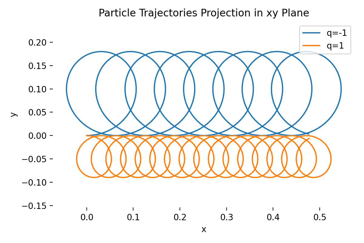
Particle trajectories projection in xy plane for two particles with opposite charges but different masses, starting with initial velocity v0=(0.1,0,0) in the presence of a small electric field in y direction and a uniform magnetic field in z direction.

As we can see from the plot, both particles gyrate around the magnetic field lines, but their gyroradii differ due to their different masses. The presence of the electric field causes both particles to drift. Since the electric field is in the y-direction and the magnetic field is in the z-direction, both particles experience a drift in the x-direction due to the $\mathbf{E}\times\mathbf{B}$ drift. The drift velocity is the same for both particles, as expected:

\[\mathbf{v}_{E\times B} = \frac{\mathbf{E} \times \mathbf{B}}{B^2} = \frac{(0,0.01,0) \times (0,0,1)}{1^2} = (0.01, 0, 0).\]

There is no motion along the z-axis since the initial velocity in that direction is zero:

plot_trajectories([X1, X3], title=f"Particle Trajectories for q and -q w/ v0={v0}",
                  plotname=f"particle_trajectories_v0_{v0[0]}_{v0[1]}_{v0[2]}.png")
plt.close()

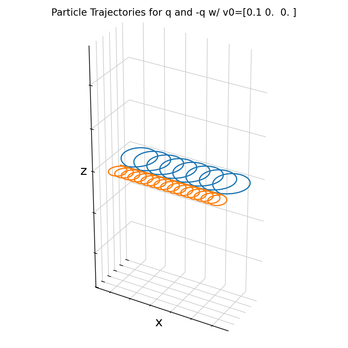
Same particle trajectories as above, but visualized in 3D. Both particles gyrate around the magnetic field lines while drifting in the x direction due to the E×B drift. There is no motion along the z-axis since the initial velocity in that direction is zero.

The particles’ velocity therefore consists of only two components:

Gyromotion around the magnetic field lines, and
E×B drift perpendicular to both E and B fields.

As soon as we give a little pinch of initial velocity along the magnetic field lines (i.e., v0_z ≠ 0), the particles will also move along the z-axis, resulting in helical trajectories:

v0 = np.array((0.1,0,0.1)) 

t1, X1 = calc_trajectory(   qe1, me1, r0=(0,0,0), v0=v0, E=E, B=B)
t3, X3 = calc_trajectory(  -qe2, me2, r0=(0,0,0), v0=v0, E=E, B=B)

plot_trajectories([X1, X3], title=f"Particle Trajectories for q and -q w/ v0={v0}",
                  plotname=f"particle_trajectories_v0_{v0[0]}_{v0[1]}_{v0[2]}.png")
plt.close()

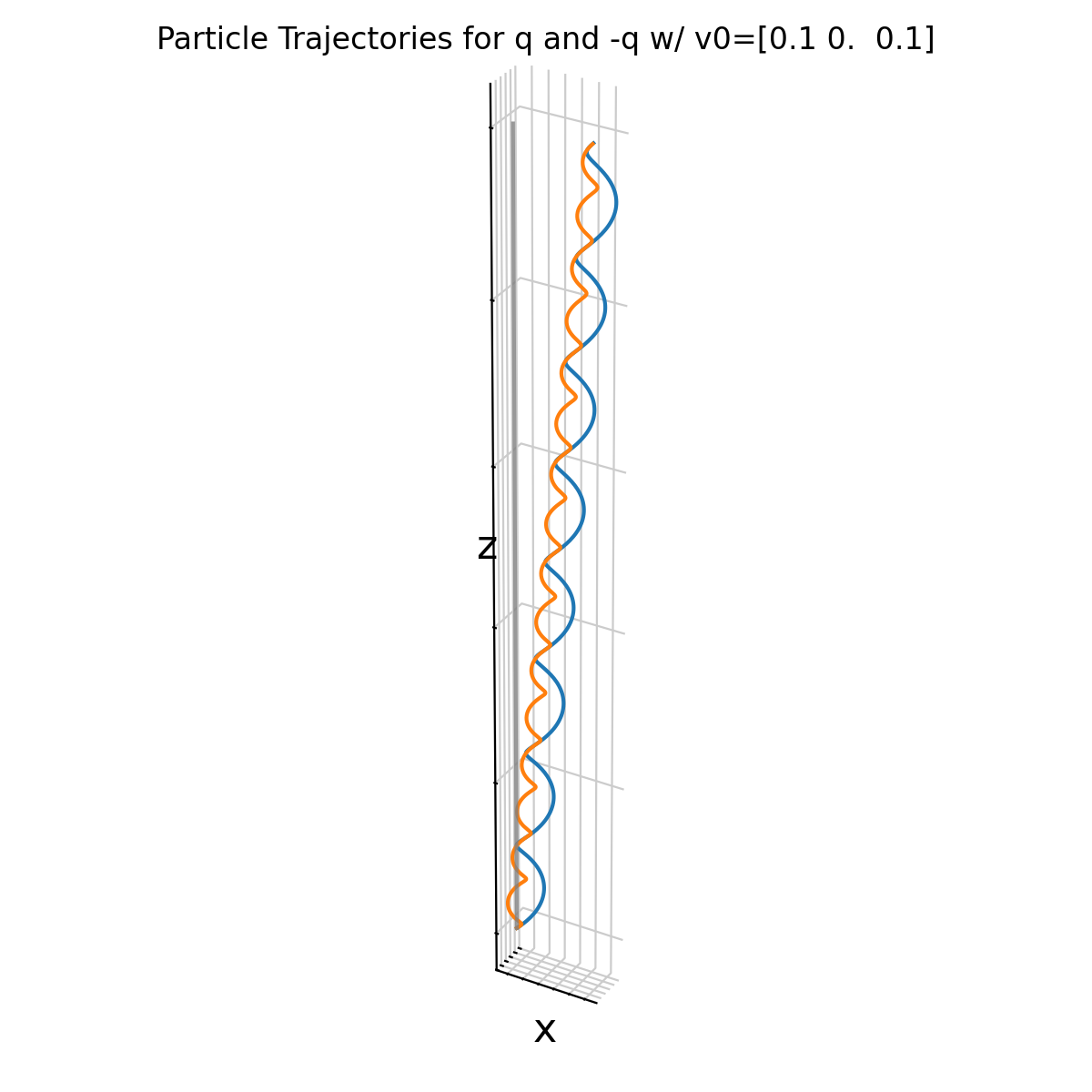
Same simulation as above, but now with a small initial velocity component along the magnetic field lines (v0_z=0.1). The particles now follow helical trajectories around the magnetic field lines while drifting in the x direction due to the E×B drift.

Animation of gyration with guiding center motion

The original tutorial scipython.comꜛ included a cool animation of the particle gyration. I simply extended it here with guiding center motion and the helix axis. Let’s begin by defining a new set of parameters for the particles and fields and turning off the electric field for simplicity (we will try different E field values later):

# charges and masses of the electron (e) and ion (i); we assume normalized units:
qe, me = -1, 1
qi, mi = 1, 3
v0=np.array((1,0,1))

E = np.array((0,0.00,0))
#E = np.array((0,0.05,0)) # try different E field values; here: particles will have an E×B drift
#E = np.array((0,0.15,0))
B = np.array((0,0.00,1))

We again calculate the trajectories for both particles:

te, Xe = calc_trajectory(qe, me, E=E, B=B, v0=v0)
ti, Xi = calc_trajectory(qi, mi, E=E, B=B, v0=v0)

We do not plot the full trajectories right away, but instead prepare some quantities needed for the animation. First, we precompute the guiding center trajectories for both particles:

B_sq = float(B @ B)
V_EB = np.cross(E, B) / B_sq # constant drift velocity
# initial guiding center position (at t=0) and guiding center trajectory:
Rgc0 = np.array([0.0, 0.0, 0.0])
Rgc_e = Rgc0[None, :] + te[:, None] * V_EB[None, :]
Rgc_i = Rgc0[None, :] + ti[:, None] * V_EB[None, :]

For the animation, we also need to calculate the axis limits based on the full trajectories of both particles:

# calculate axis limits:
XYZ = np.vstack((Xe[:, :3], Xi[:, :3]))
mins = XYZ.min(axis=0)
maxs = XYZ.max(axis=0)
marg = 0.05 * (maxs - mins + 1e-12)
xmin, ymin, zmin = mins - marg
xmax, ymax, zmax = maxs + marg

We also want to visualize the helix axis of each particle, which combines the guiding center drift and the parallel motion along the magnetic field lines. The helix axis corresponds to the trajectory of the guiding center augmented by the constant parallel motion along $\mathbf{B}$. Thus, we calculate:

# calculate the helix axis:
bhat = B / np.linalg.norm(B) # # unit vector along B
# parallel velocities (constant in homogeneous fields):
vpar_e = float(np.dot(Xe[0, 3:], bhat))
vpar_i = float(np.dot(Xi[0, 3:], bhat))
# helix axes: perpendicular guiding center drift + parallel transport
Raxis_e = Rgc_e + (te[:, None] * vpar_e) * bhat[None, :]
Raxis_i = Rgc_i + (ti[:, None] * vpar_i) * bhat[None, :]

Now we define two functions for initializing and updating the animation frames:

def init():
    fig = plt.figure()
    ax = fig.add_subplot(111, projection="3d")

    ax.set_xlim(xmin, xmax)
    ax.set_ylim(ymin, ymax)
    ax.set_zlim(zmin, zmax)
    ax.set_box_aspect((xmax-xmin, ymax-ymin, zmax-zmin))
    ax.view_init(elev=25, azim=-60)

    # reference B direction line through origin; when E=0, this is 
    # also guiding center line of the gyro-motion; if E≠0, it's at
    #  the GC at t=0; along z):
    ax.plot([0,0],[0,0],[zmin, zmax], lw=2, c="gray", alpha=0.6,
            label="magnetic field direction")

    # start empty, not full trajectories for electron motion, ion motion:
    lne, = ax.plot([], [], [], c="tab:blue", lw=2, label="electron")
    lni, = ax.plot([], [], [], c="tab:orange", lw=2, label="ion")
    dGC  = ax.plot([], [], [], "ok", label="guiding center") # dummy plot for legend of guiding center

    # plot the particles instantaneous positions as a scatter plot, scaled
    # according to particle mass:
    SCALE = 40
    particles = ax.scatter(*np.vstack((Xe[0][:3], Xi[0][:3])).T,
                           s=(me*SCALE, mi*SCALE),
                           c=("tab:blue", "tab:orange"), depthshade=0)

    # plot guiding center (GC) points (two black dots):
    gc_scatter = ax.scatter([Rgc_e[0,0], Rgc_i[0,0]],
                            [Rgc_e[0,1], Rgc_i[0,1]],
                            [Rgc_e[0,2], Rgc_i[0,2]],
                            s=25, c="k", depthshade=0)

    # plot helix axis traces (also time evolving):
    axis_e_line, = ax.plot([], [], [], "--", lw=1.5, alpha=0.6, c="tab:blue",
                           label="helix axis (electron)")
    axis_i_line, = ax.plot([], [], [], "--", lw=1.5, alpha=0.6, c="tab:orange",
                           label="helix axis (ion)")
    # add current point on each helix axis (x markers):
    axis_pts = ax.scatter([Raxis_e[0,0], Raxis_i[0,0]],
                          [Raxis_e[0,1], Raxis_i[0,1]],
                          [Raxis_e[0,2], Raxis_i[0,2]],
                          s=20, c=("tab:blue", "tab:orange"), marker="o", depthshade=0,
                          alpha=0.6)

    # add some title info including E and B fields:
    ax.set_title("Numerical integration of particle motion\n"
                 f"E = ({E[0]:.2f}, {E[1]:.2f}, {E[2]:.2f}), "
                 f"B = ({B[0]:.2f}, {B[1]:.2f}, {B[2]:.2f})\n")
    
    # add a legend:
    ax.legend(loc="upper right", bbox_to_anchor=(1.35, 1.0))
    
    # apply custom axes function:
    setup_axes(ax)

    return fig, ax, lne, lni, particles, gc_scatter, axis_e_line, axis_i_line, axis_pts

def animate(i):    
    # update electron and ion trajectories up to step i:
    lne.set_data(Xe[:i,0], Xe[:i,1])
    lne.set_3d_properties(Xe[:i,2])

    lni.set_data(Xi[:i,0], Xi[:i,1])
    lni.set_3d_properties(Xi[:i,2])

    # update particle positions:
    particles._offsets3d = np.vstack((Xe[i][:3], Xi[i][:3])).T

    # also indicate the current guiding center position of each particle
    # on the xy plane (z=0); actually two points, but usually overlapping:
    gc_scatter._offsets3d = np.array([[Rgc_e[i,0], Rgc_i[i,0]],
                                      [Rgc_e[i,1], Rgc_i[i,1]],
                                      [Rgc_e[i,2], Rgc_i[i,2]]])
    
    # plot helix axis lines up to current time:
    axis_e_line.set_data(Raxis_e[:i, 0], Raxis_e[:i, 1])
    axis_e_line.set_3d_properties(Raxis_e[:i, 2])
    axis_i_line.set_data(Raxis_i[:i, 0], Raxis_i[:i, 1])
    axis_i_line.set_3d_properties(Raxis_i[:i, 2])

    # indicate current helix-axis points (also two points, but usually overlapping):
    axis_pts._offsets3d = np.array([[Raxis_e[i,0], Raxis_i[i,0]],
                                    [Raxis_e[i,1], Raxis_i[i,1]],
                                    [Raxis_e[i,2], Raxis_i[i,2]]])

    # add a time stamp:
    time_text = f"t = {te[i]:.2f}" # unitless time (!)
    if not hasattr(animate, "time_annotation"):
        animate.time_annotation = ax.text2D(0.05, 0.95, time_text, transform=ax.transAxes)
    else:
        animate.time_annotation.set_text(time_text)

Now, we have everything at hand to create and save the animation (here, as an mp4 video file):

print("animating...")
fig, ax, lne, lni, particles, gc_scatter, axis_e_line, axis_i_line, axis_pts = init()
anim = animation.FuncAnimation(fig, animate, frames=len(te), interval=10, blit=False)
HTML(anim.to_html5_video())
plt.tight_layout()
# save animation as mp4 video file:
anim.save(f'gyration_animation_E{E[1]:.2f}_B{B[1]:.2f}.mp4', writer='ffmpeg', fps=30, dpi=200)
plt.close()
print("animation complete.")

Animation of the particle gyration in the presence of uniform magnetic field. The blue and orange lines represent the trajectories of an electron and an ion, respectively. The black dots indicate the guiding center positions (overlap for both particles), while the dashed lines show the helix axes (also overlap for both particles). The magnetic field direction is indicated by the gray vertical line. Here, no electric field is present (E=0), so there is no E×B drift.

In our above simulation, we hade no electric field present (E=0), so there was no E×B drift, so that the guiding center and helix axis of both particles overlap and remain at the origin in the xy plane. The particles’ motion is purely helical around the magnetic field lines and consists of two components:

Gyromotion around the magnetic field lines, and
Parallel motion along the magnetic field lines.

You can try different values of the electric field,e.g., E=(0,0.15,0), in the code above to see how the trajectories change:

Same simulation as above, but now with a finite electric field in y direction (E=(0,0.15,0)). The guiding center and helix axis of both particles now drift in the x-direction due to the E×B drift.

Now, the electric field causes an E×B drift in the x-direction, which is visible as a drift of the particles along the x-axis. Also the guiding center and helix axis now drift in the x-direction. The particles’ motion now consists of three components:

Gyromotion around the magnetic field lines,
Parallel motion along the magnetic field lines, and
E×B drift perpendicular to both E and B fields.

Pitch angle experiments

In the previous examples, the initial velocity implicitly fixed the pitch angle. Here we explicitly parametrize the initial velocity by the pitch angle $\alpha$, defined as the angle between the velocity vector and the magnetic field direction:

alpha = np.radians(30) # pitch angle in degrees
v0_mag = 0.1 # magnitude of initial velocity
v0 = v0_mag * np.array([np.sin(alpha), 0.0, np.cos(alpha)])

# define some charges and masses of the electron (e) and ion (i):
qe, me = -1, 1
qi, mi = 1, 3

E = np.array((0,0.00,0))
B = np.array((0,0.00,1))

# calculate the trajectories for the particles:
te, Xe = calc_trajectory(qe, me, E=E, B=B, v0=v0)
ti, Xi = calc_trajectory(qi, mi, E=E, B=B, v0=v0)

# make a static 3D plot of the trajectories:
plot_trajectories([Xe, Xi], title=f"Particle Trajectories with Pitch Angle {np.degrees(alpha):.1f}°",
                  plotname=f"particle_trajectories_pitch_angle_{np.degrees(alpha):.1f}_deg.png")

Here are some examples of particle trajectories for different pitch angles (30°, 45°, and 75°) in the absence of an electric field:

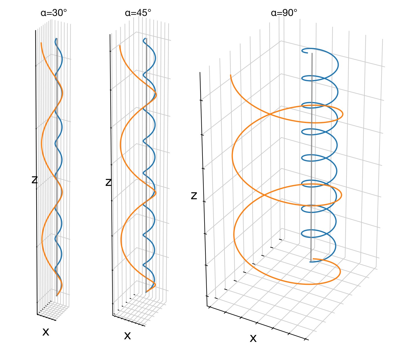
Examples of particle trajectories for different pitch angles (30°, 45°, and 75°) in the absence of an electric field. As the pitch angle increases, the particles exhibit more pronounced gyration around the magnetic field lines, while the parallel motion along the field lines decreases (the latter is hardly visible in these plots as we haven’t scalled the z-axis equally).

By parametrizing the initial velocity through the pitch angle, the geometric meaning of helical motion becomes explicit. Large pitch angles correspond to tightly wound helices with small parallel displacement, while small pitch angles produce shallow helices that propagate rapidly along magnetic field lines. This becomes even more obvious when we set the pitch angle to 90° (purely perpendicular initial velocity):

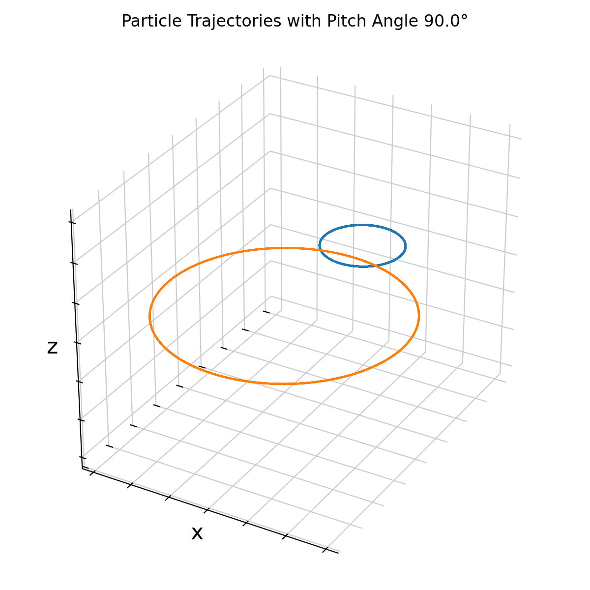
With a pitch angle of 90° (purely perpendicular initial velocity), the particles exhibit pure gyration around the magnetic field lines without any parallel motion along the field lines.

For pitch angles larger than $90^\circ$, the parallel velocity reverses sign, leading to motion in the opposite direction along the magnetic field, while the sense of gyration remains fixed by the particle charge:

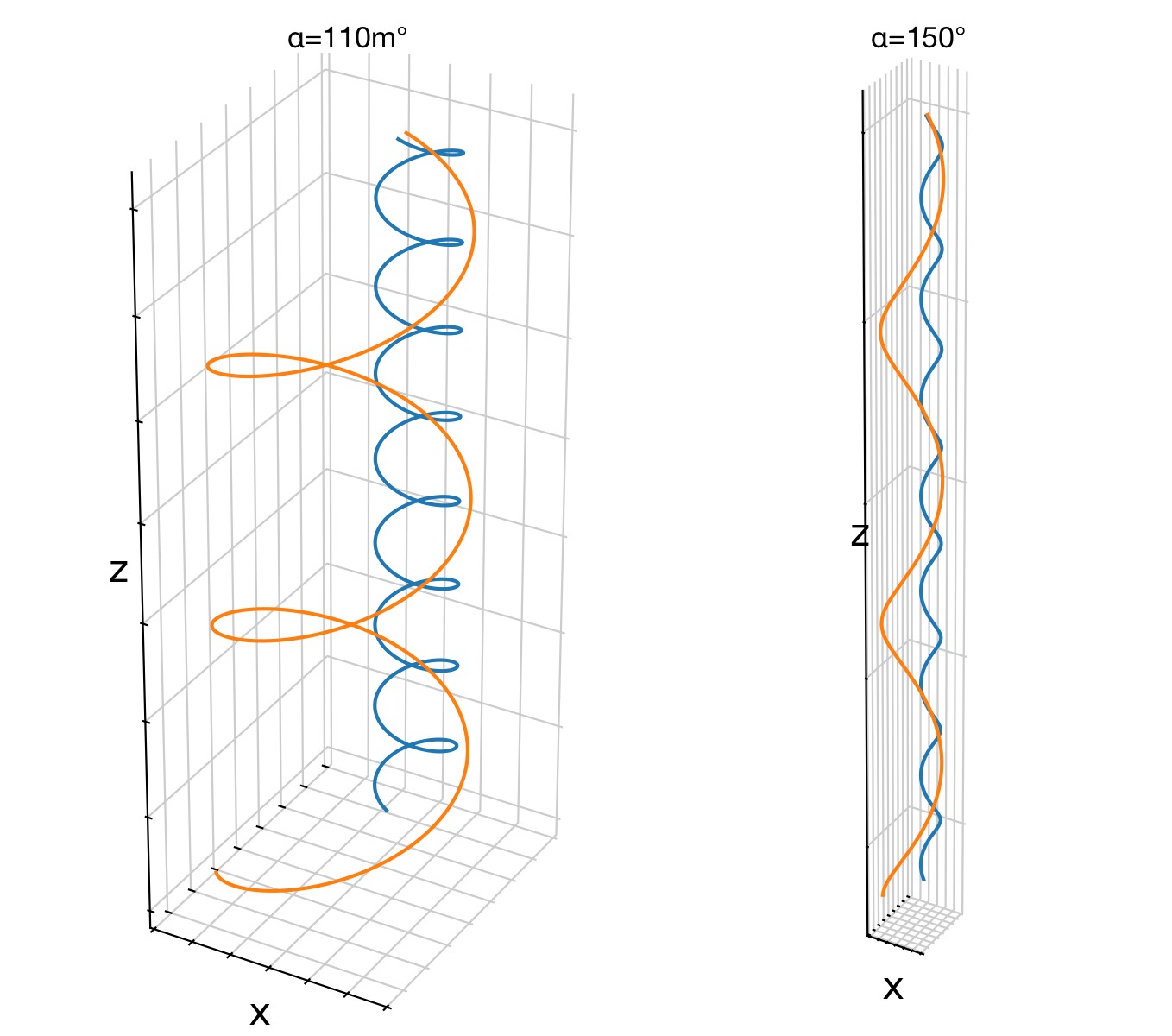
With a pitch angle of 110° and 150°, the particles gyrate in the opposite direction around the magnetic field lines while still moving parallel to the field lines.

For a pitch angle of 0° or 180°, the particles move purely along the magnetic field lines without any gyration (not shown here).

In homogeneous fields and in the absence of parallel electric fields, the pitch angle remains constant in time.

Update and code availability: This post and its accompanying Python code were originally drafted in 2020 and archived during the migration of this website to Jekyll and Markdown. In January 2026, I substantially revised and extended the code. The updated and cleaned-up implementation is now available in this new GitHub repositoryꜛ. Please feel free to experiment with it and to share any feedback or suggestions for further improvements.

References and further reading

Wolfgang Baumjohann and Rudolf A. Treumann, Basic Space Plasma Physics, 1997, Imperial College Press, ISBN: 1-86094-079-X
J. A. Bittencourt, Fundamentals of Plasma Physics, 2004, Springer, ISBN: 978-0-387-20975-3
Wikipedia article on Plasmaꜛ
Wikipedia article on Plasma gyromotionꜛ