The solar wind and the Parker model

August 21, 2020 January 23, 2026 23 minute read see also comments

The solar wind is a continuous, supersonic outflow of ionized plasma from the solar corona into interplanetary space. Its existence and basic properties are now observationally well established, yet its theoretical understanding originates from a remarkably simple hydrodynamic argument developed in the late 1950s by Eugene Parker. Parker’s model not only explains why the corona cannot remain static but also predicts the large scale structure of the interplanetary magnetic field, now known as the Parker spiral.

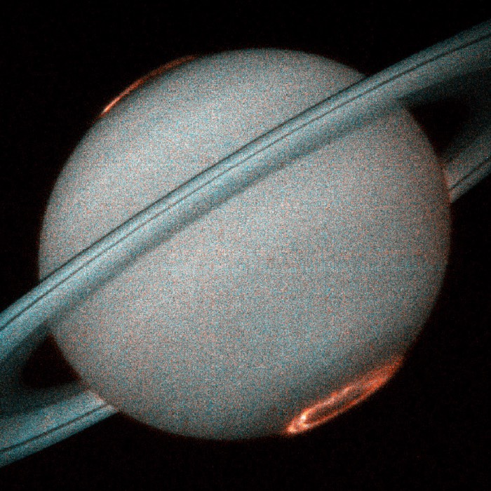
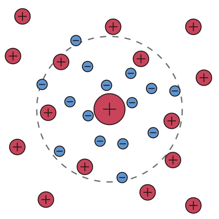
Artist’s impression of solar wind flow around Earth’s magnetosphere. The solar wind is a continuous outflow of ionized plasma from the Sun that interacts with planetary magnetic fields. Source: Wikimedia Commonsꜛ (license: public domain).

In this post, we present a compact introduction to the Parker solar wind model and the resulting spiral geometry of the heliospheric magnetic field. We complete this brief theoretical overview with a simple numerical experiment that simulates the Parker spiral structure with a simple Python code.

Physical picture

The Sun rotates, while the hot coronal plasma expands radially outward. Because the solar plasma is highly conducting, the magnetic field is frozen into the flow to very good approximation. Magnetic field lines emerging from the corona therefore remain magnetically connected to the rotating Sun while being advected outward by the solar wind.

Illustration of the Parker spiral structure of the solar magnetic field in the ecliptic plane, caused by the interaction between the radially outward solar wind and the Sun’s rotation. Source: Wikimedia Commonsꜛ (license: public domain).

An observer in an inertial frame thus does not see purely radial magnetic field lines. Instead, the combined effect of solar rotation and radial outflow bends the field into a spiral pattern. A helpful analogy is water emitted from a rotating garden sprinkler: although the water leaves the nozzle radially, the rotation of the source curves the trajectory. In the heliosphere, this curvature takes the form of an Archimedean spiral.

Hydrodynamic Parker model of the solar wind

The Parker model describes the solar wind as a stationary, radially symmetric plasma outflow under solar gravity and pressure forces. The key assumptions are strong stationarity, $\partial_t = 0$, but not static equilibrium, and spherical symmetry.

Continuity equation

For a steady, spherically symmetric flow with radial velocity $\mathbf{v} = v(r),\widehat{\mathbf{e}}_r$,where $\widehat{\mathbf{e}}_r$ is the radial unit vector, the continuity equation reads

\[\begin{align} \nabla \cdot (\rho \mathbf{v}) = 0 \end{align}\]

which in spherical coordinates reduces to

\[\begin{align} \frac{1}{r^2},\partial_r \left(r^2 \rho v\right) = 0. \end{align}\]

This expresses conservation of mass flux through spherical shells.

Radial momentum equation

The radial equation of motion for the plasma in the solar gravitational field is

\[\begin{align} v,\partial_r v = -\frac{G M_{\odot}}{r^2} - \frac{1}{\rho},\partial_r p, \end{align}\]

where $M_{\odot}$ is the solar mass, $\rho = m n$ the mass density, $p$ the thermal pressure, and $G$ the gravitational constant.

To close the system, a polytropic relation between pressure and density is assumed,

\[\begin{align} \frac{p}{n^{\gamma}} = \text{const.}, \end{align}\]

with $1 < \gamma \leq 5/3$. In the simplest and analytically tractable case, the isothermal approximation $\gamma = 1$ is adopted. The pressure gradient then satisfies

\[\begin{align} \partial_r p = c_S^2,\partial_r \rho, \end{align}\]

where $c_S$ is the isothermal sound speed.

Substituting into the momentum equation and combining with the continuity equation yields

\[\begin{align} \frac{1}{v},\partial_r v,(v^2 - c_S^2) = -\frac{G M_{\odot}}{r^2} + \frac{2 c_S^2}{r}. \end{align}\]

Critical solution

This differential equation admits multiple solution branches depending on boundary conditions. Only one solution is physically meaningful: The transonic solution that passes smoothly through a critical radius where $v = c_S$. This solution accelerates from subsonic speeds near the Sun to supersonic velocities at large distances and is fully consistent with in situ measurements of the solar wind.

All other solution branches either decelerate unphysically or fail to connect the corona to interplanetary space. The existence of a unique transonic solution is the central result of Parker’s theory.

Plasma beta and magnetic field advection

Beyond the critical radius, the solar wind speed approaches an approximately constant value $v_0$. The orientation of the interplanetary magnetic field is then governed by the competition between plasma dynamics and magnetic forces.

This balance is quantified by the plasma beta,

\[\begin{align} \beta = \frac{2 \mu_0 p}{B^2}, \end{align}\]

the ratio of thermal to magnetic pressure. In the solar wind, $\beta$ is typically of order 10 to 20, indicating that thermal pressure dominates over magnetic tension. As a consequence:

the flow remains nearly radial,
the magnetic field is advected by the plasma,
magnetic forces do not significantly alter the large scale flow geometry.

These conditions justify treating the magnetic field as passively frozen into the radial outflow.

Geometry of the Parker spiral

Let the Sun rotate with angular velocity $\Omega$, and consider a plasma element launched radially outward at speed $v_0$. The azimuthal position of the magnetic field line connected to that plasma element evolves as

\[\begin{align} \varphi_P = \varphi + \Omega (t - t_\varphi). \end{align}\]

Eliminating time using $r = r_0 + v_0 (t - t_\varphi)$ leads to

\[\begin{align} r = r_0 + \frac{v_0}{\Omega} (\varphi_P - \varphi), \end{align}\]

which is the equation of an Archimedean spiral. This curve defines the Parker spiral structure of the heliospheric magnetic field.

Magnetic field components

The spiral geometry directly constrains the magnetic field components. The Parker angle $\phi$, defined as the angle between the magnetic field and the radial direction, satisfies

\[\begin{align} \tan(\phi) = -\frac{B_\varphi}{B_r}. \end{align}\]

From the spiral geometry,

\[\begin{align} \frac{B_r}{B_\varphi} = \frac{dr}{r,d\varphi} = \frac{v_0}{\Omega r}, \end{align}\]

which gives

\[\begin{align} B_\varphi = - B_r \frac{\Omega r}{v_0}, \qquad \tan(\phi) = \frac{\Omega r}{v_0}. \end{align}\]

Using $\nabla \cdot \mathbf{B} = 0$ under radial symmetry yields

\[\begin{align} B_r = B_0 \left(\frac{R_0}{r}\right)^2, \end{align}\]

and therefore

\[\begin{align} B_\varphi = - B_0 \frac{R_0^2}{r},\frac{\Omega}{v_0}. \end{align}\]

These expressions fully characterize the large scale interplanetary magnetic field in the Parker model.

Numerical simulations with Python

Before introducing time-discrete or particle-based simulations, it is instructive to visualize the Parker spiral directly from its analytical expression. This approach implements Parker’s solution in its closed form and therefore serves as a clean reference against which more elaborate numerical models can later be compared.

Analytical visualization of the Parker spiral

Physical assumptions

The analytical implementation rests on the same idealized assumptions as the classical Parker model:

the solar wind flows radially outward with a constant speed $v_{\mathrm{sw}}$ for $r \ge r_0$,
the Sun rotates rigidly with a constant angular velocity $\Omega$,
the plasma is highly conducting, so that the magnetic field is frozen into the flow,
magnetic forces do not significantly modify the bulk flow, consistent with a high plasma beta.

Under these conditions, magnetic field lines are passively advected by the solar wind while remaining magnetically connected to their rotating footpoints at the Sun.

Field-line mapping

Consider a magnetic field line whose footpoint has inertial longitude $\phi_0$ at time $t = 0$. A plasma element currently located at radial distance $r$ at time $t$ must have left the source surface at an earlier time

\[t_{\mathrm{launch}} = t - \frac{r - r_0}{v_{\mathrm{sw}}}.\]

At that launch time, the solar footpoint had rotated to the longitude

\[\phi_{\mathrm{foot}}(t_{\mathrm{launch}}) = \phi_0 + \Omega, t_{\mathrm{launch}}.\]

Because of flux freezing, the plasma element preserves this longitude during its radial propagation. The azimuthal position of the field line at radius $r$ and time $t$ is therefore

\[\begin{align*} \phi(r,t) &= \phi_0 + \Omega\left(t - \frac{r - r_0}{v_{\mathrm{sw}}}\right) \\ &= (\phi_0 + \Omega t) - \frac{\Omega}{v_{\mathrm{sw}}}(r - r_0). \end{align*}\]

This relation defines an Archimedean spiral in polar coordinates $(r,\phi)$ and represents the Parker spiral in its simplest analytical form.

Numerical implementation strategy

Our Python implementation below evaluates this expression directly. For each time step, a set of field lines with different initial footpoint longitudes $\phi_0$ is drawn by sampling the radial coordinate between $r_0$ and a chosen outer boundary $r_{\max}$. The resulting curves are plotted in polar coordinates, producing one clean Parker spiral per time step.

Although the visualization is time-dependent, no dynamical evolution is solved numerically. Time enters only as a parameter that shifts the spiral through the term $\Omega t$. In this sense, the code visualizes a family of exact solutions rather than performing a simulation in the strict numerical sense.

Purpose and interpretation

This analytical rendering serves three didactic purposes:

First, it provides a direct visualization of Parker’s solution without additional numerical assumptions. Every feature of the spiral can be traced back to a specific term in the analytical expression.

Second, it makes the dependence on physical parameters transparent. Changes in solar wind speed, rotation rate, or source radius immediately translate into predictable modifications of the spiral geometry.

Third, it establishes a clear baseline for more advanced models. In later sections, the same spiral structure will be reconstructed from time-discrete plasma parcels and ballistic propagation. The agreement between both approaches highlights that the Parker spiral is not an imposed geometry, but an inevitable consequence of radial outflow combined with solar rotation.

In this sense, the analytical implementation is best understood as a visualization of theory, while subsequent numerical approaches demonstrate how the same structure emerges dynamically from plasma motion.

Python code

from __future__ import annotations

import os
import math
from dataclasses import dataclass

import numpy as np
import matplotlib.pyplot as plt

import imageio.v2 as imageio

# define constants:
AU = 1.495978707e11  # m, astronomical unit
R_SUN = 6.9634e8     # m, solar radius

# define parameters dataclass that holds all simulation settings:
@dataclass
class ParkerAnalyticParams:
    v_sw: float = 400e3          # m/s
    omega: float = 2.86533e-6    # rad/s
    r0: float = 10.0 * R_SUN     # m
    r_max: float = 2.0 * AU      # m

    n_lines: int = 12            # number of spirals with different phi0
    n_r: int = 2000              # resolution along r

    dt: float = 6 * 3600.0       # s
    n_steps: int = 80            # number of frames

    # plot styling:
    figsize: tuple[float, float] = (7.0, 7.0)
    dpi: int = 170

# function to ensure output directory exists:
def ensure_dir(path: str) -> None:
    os.makedirs(path, exist_ok=True)

# function to wrap angles to [-pi, pi]:
def wrap_pi(a: np.ndarray) -> np.ndarray:
    """Wrap angles to [-pi, pi] for nicer polar plotting."""
    return (a + np.pi) % (2.0 * np.pi) - np.pi

# function to render frames of the Parker spiral:
def render_parker_spiral_frames(
    params: ParkerAnalyticParams,
    out_dir: str = "frames_parker_spiral_clean",
    make_gif: bool = False,
    gif_path: str = "parker_spiral_clean.gif",
    gif_frame_duration_s: float = 0.08) -> None:
    ensure_dir(out_dir)

    # radii to draw (meters):
    r = np.linspace(params.r0, params.r_max, params.n_r)

    # choose evenly spaced field-line footpoint longitudes at t=0:
    phi0s = np.linspace(0.0, 2.0 * np.pi, params.n_lines, endpoint=False)

    gif_frames = []

    for k in range(params.n_steps):
        t = k * params.dt

        fig = plt.figure(figsize=params.figsize)
        ax = fig.add_subplot(111, projection="polar")

        # reference circles: Sun radius and r0:
        theta_ref = np.linspace(-np.pi, np.pi, 512)
        ax.plot(theta_ref, np.full_like(theta_ref, R_SUN / AU), linewidth=1.0)
        ax.plot(theta_ref, np.full_like(theta_ref, params.r0 / AU), linewidth=1.0)

        # Draw each spiral
        for phi0 in phi0s:
            phi = phi0 + params.omega * t - (params.omega / params.v_sw) * (r - params.r0)
            theta = wrap_pi(phi)
            ax.plot(theta, r / AU, linewidth=1.3)

        ax.set_rlim(0.0, params.r_max / AU)
        ax.set_rlabel_position(135)

        ax.set_title(
            "Parker spiral (analytic curve)\n"
            f"t = {t/3600:.1f} h, v_sw = {params.v_sw/1e3:.0f} km/s, Ω = {params.omega:.2e} rad/s",
            va="bottom")

        frame_path = os.path.join(out_dir, f"frame_{k:05d}.png")
        fig.savefig(frame_path, dpi=params.dpi, bbox_inches="tight")
        plt.close(fig)

        if make_gif:
            try:
                import imageio.v2 as imageio
            except Exception as e:
                raise RuntimeError("make_gif=True requires imageio. Install via: pip install imageio") from e
            gif_frames.append(imageio.imread(frame_path))

    # assemble GIF:
    if make_gif:
        import imageio.v2 as imageio
        imageio.mimsave(gif_path, gif_frames, duration=gif_frame_duration_s)
        print(f"Wrote GIF: {gif_path}")

    print(f"Wrote {params.n_steps} frames to: {out_dir}")

# main:
if __name__ == "__main__":
    params = ParkerAnalyticParams(
        v_sw=400e3,         # 400 km/s
        omega=2.865e-6,     # rad/s
        r0=10 * R_SUN,
        r_max=2.0 * AU,
        n_lines=14,
        n_r=2500,
        dt=6 * 3600.0,
        n_steps=90,
        dpi=180)

    render_parker_spiral_frames(
        params,
        out_dir="frames_parker_spiral_analytic",
        make_gif=True,
        gif_path="parker_spiral_analytic.gif",
        gif_frame_duration_s=0.08)

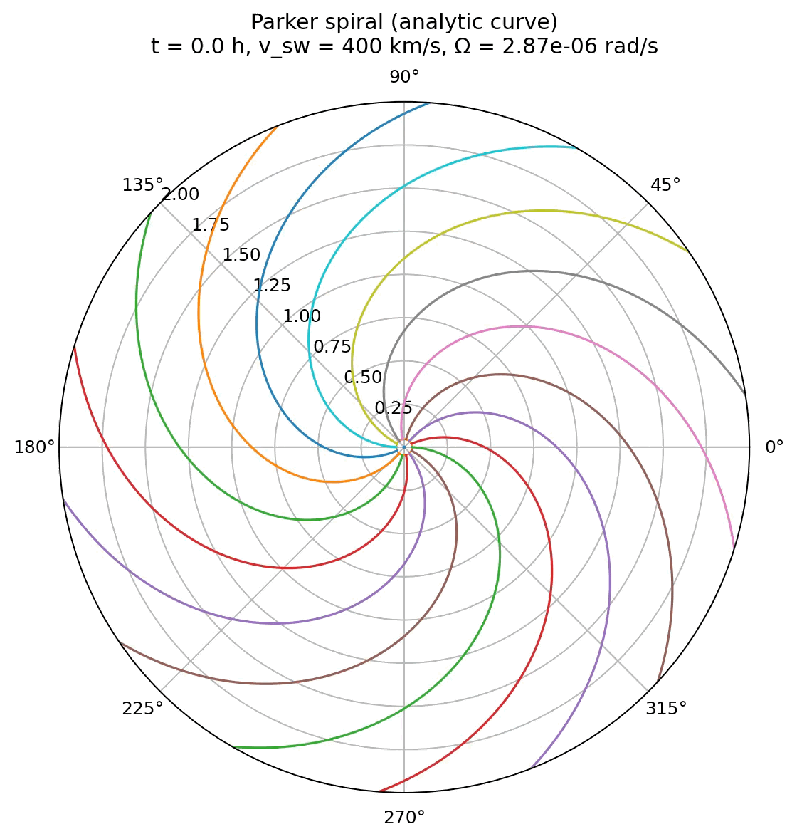
Simulation of the Parker spiral structure of the interplanetary magnetic field using the analytical expression for field line mapping. The spiral is drawn for a solar wind speed of 400 km/s and a source surface at 10 solar radii.

The animation generated from the analytical implementation shows the Parker spiral as a sequence of exact, closed curves, each corresponding to a different observation time. The spiral does not evolve dynamically in the sense of a physical simulation. Instead, time acts as a parameter that shifts the solution through the term $\Omega t$ in the analytical expression for $\phi(r,t)$.

This visualization highlights the purely geometric origin of the Parker spiral. For a given solar wind speed and rotation rate, the spiral shape is fully determined and exists at all times. The apparent rotation of the pattern reflects the continuous rotation of the solar footpoints, not the motion of individual plasma elements along the field line. As a result, the spiral appears smooth, stationary in shape, and free of transient features.

This animation emphasizes that the Parker spiral is an unavoidable consequence of steady radial outflow combined with solar rotation. It provides a clear reference solution against which more dynamical or numerical approaches can be compared. Any deviation from this shape in more advanced models can therefore be directly attributed to additional physics rather than to the basic Parker mechanism itself.

Ballistic reconstruction of the Parker spiral

After visualizing the Parker spiral directly from its analytical expression, as a next step we reconstruct the same structure from an explicit time evolution of plasma parcels. Our next implementation does not draw the spiral as a closed curve, but lets it emerge dynamically from the combined effects of solar rotation and radial plasma outflow.

Physical interpretation

The underlying physical assumptions are identical to those of the analytical model. The solar wind is treated as a steady, radial flow with constant speed $v_{\mathrm{sw}}$, originating at a source surface of radius $r_0$. The Sun rotates rigidly with angular velocity $\Omega$, and the plasma is assumed to be perfectly conducting, so that the magnetic field is frozen into the flow. Magnetic forces are neglected at leading order, consistent with a high plasma beta in the solar wind.

The key conceptual shift is that magnetic field lines are no longer treated as geometric objects. Instead, they are reconstructed from the trajectories of many individual plasma elements that were launched from the rotating Sun at different times.

Launch and propagation of plasma parcels

For each magnetic footpoint longitude $\phi_0$, the code repeatedly launches plasma parcels from the source radius $r_0$. At a given simulation time $t$, the footpoint has rotated to the longitude

\[\phi_{\mathrm{foot}}(t) = \phi_0 + \Omega t.\]

A newly launched parcel is assigned this longitude and then propagates radially outward with constant speed $v_{\mathrm{sw}}$. Its radial position at a later time $t$ is therefore

\[r(t) = r_0 + v_{\mathrm{sw}} (t - t_{\mathrm{launch}}),\]

where $t_{\mathrm{launch}}$ denotes the launch time of the parcel. Because of flux freezing, the parcel preserves the longitude it had at launch throughout its motion.

At any given simulation time, the spatial distribution of all previously launched parcels associated with the same footpoint traces out a magnetic field line. The Parker spiral thus appears as the envelope of many radially streaming plasma elements whose launch longitudes continuously change due to solar rotation.

Numerical structure of the model

The simulation proceeds in discrete time steps of size $\Delta t$. At each step, new plasma parcels are injected at the source surface for each footpoint longitude. Previously launched parcels are advanced ballistically according to the radial flow. Parcels that move beyond a predefined outer radius are discarded to limit the computational domain.

The model is two dimensional and restricted to the ecliptic plane. No forces are integrated numerically. The dynamics are purely kinematic and follow directly from the prescribed flow speed and rotation rate. Time enters explicitly through the launch history of the plasma parcels.

For visualization, the positions of all parcels are plotted in polar coordinates at each time step. This produces a sequence of frames that show the gradual formation and outward transport of the Parker spiral. The frames can be saved individually or assembled into an animated image.

Python code

from __future__ import annotations

import os
import math
from dataclasses import dataclass

import numpy as np
import matplotlib.pyplot as plt

import imageio.v2 as imageio
# %% CONSTANTS
AU = 1.495978707e11  # m
R_SUN = 6.9634e8     # m


# define parameters dataclass that holds all simulation settings:
@dataclass
class ParkerSpiralParams:
    # solar wind speed (constant):
    v_sw: float = 400e3  # m/s

    # solar rotation rate (sidereal ~ 25.38 days at equator):
    # You can also use synodic ~ 27.27 days:
    omega: float = 2.86533e-6  # rad/s

    # launch radius (start of spiral), e.g. a few solar radii:
    r0: float = 10.0 * R_SUN  # m

    # max plotting radius (domain):
    r_max: float = 2.0 * AU  # m

    # number of distinct field lines (different longitudes):
    n_lines: int = 16

    # initial longitudes for the lines at t=0 (if None: uniform):
    phi0: np.ndarray | None = None

    # simulation time settings:
    dt: float = 6 * 3600.0  # s (6 hours)
    n_steps: int = 80

    # launch cadence for new parcels per line 
    # (smaller => smoother spirals, heavier compute):
    launch_every: int = 1  # launch each step

    # for each line, keep all parcels or cap for performance:
    max_parcels_per_line: int = 5000

# function to ensure output directory exists:
def ensure_dir(path: str) -> None:
    os.makedirs(path, exist_ok=True)

# function to create uniform phi0 values:
def make_phi0(n_lines: int) -> np.ndarray:
    return np.linspace(0.0, 2.0 * np.pi, n_lines, endpoint=False)

# main simulation function:
def simulate_parker_spiral(
    params: ParkerSpiralParams,
    out_dir: str = "frames_parker_spiral",
    make_gif: bool = False,
    gif_path: str = "parker_spiral.gif",
    dpi: int = 160) -> None:
    """
    Main simulation function for Parker spiral with ballistic mapping.
    """
    ensure_dir(out_dir)

    phi0 = params.phi0 if params.phi0 is not None else make_phi0(params.n_lines)
    phi0 = np.asarray(phi0, dtype=float)
    if phi0.shape != (params.n_lines,):
        raise ValueError(f"phi0 must have shape ({params.n_lines},), got {phi0.shape}")

    # for each line we store arrays of launch_times and launch_phis:
    launch_times = [np.empty(0, dtype=float) for _ in range(params.n_lines)]
    launch_phis = [np.empty(0, dtype=float) for _ in range(params.n_lines)]

    # helper: wrap angles to [-pi, pi] for plotting continuity:
    def wrap_pi(a: np.ndarray) -> np.ndarray:
        return (a + np.pi) % (2.0 * np.pi) - np.pi

    # for optional GIF assembly:
    gif_frames = []

    # precompute plot extent:
    r_plot_max_AU = params.r_max / AU

    for k in range(params.n_steps):
        t = k * params.dt

        # launch new parcels (footpoints co-rotate with the Sun):
        if (k % params.launch_every) == 0:
            for i in range(params.n_lines):
                phi_foot = phi0[i] + params.omega * t  # co-rotating footpoint
                # Append one launch
                launch_times[i] = np.append(launch_times[i], t)
                launch_phis[i] = np.append(launch_phis[i], phi_foot)

                # Cap memory if needed
                if launch_times[i].size > params.max_parcels_per_line:
                    launch_times[i] = launch_times[i][-params.max_parcels_per_line :]
                    launch_phis[i] = launch_phis[i][-params.max_parcels_per_line :]

        # build frame plot:
        fig = plt.figure(figsize=(7, 7))
        ax = fig.add_subplot(111, projection="polar")

        # plot Sun and launch radius as reference circles:
        theta_ref = np.linspace(-np.pi, np.pi, 512)
        ax.plot(theta_ref, np.full_like(theta_ref, R_SUN / AU), linewidth=1.0)
        ax.plot(theta_ref, np.full_like(theta_ref, params.r0 / AU), linewidth=1.0)

        # for each field line, compute current parcel positions:
        for i in range(params.n_lines):
            if launch_times[i].size == 0:
                continue

            tau = t - launch_times[i]  # time since launch
            # only parcels that have had time to travel outward:
            valid = tau >= 0.0
            if not np.any(valid):
                continue

            tau = tau[valid]
            phi_launch = launch_phis[i][valid]

            # ballistic mapping:
            r = params.r0 + params.v_sw * tau  # meters
            keep = r <= params.r_max
            if not np.any(keep):
                continue

            r = r[keep]
            phi = phi_launch[keep]  # frozen-in angle
            # convert to polar plot coordinates: theta = inertial longitude:
            theta = wrap_pi(phi)
            ax.plot(theta, r / AU, linewidth=1.2)

        # formatting:
        ax.set_rlim(0.0, r_plot_max_AU)
        ax.set_rlabel_position(135)
        ax.set_title(
            "Parker spiral (ballistic mapping)\n"
            f"t = {t/3600:.1f} h, v_sw = {params.v_sw/1e3:.0f} km/s, "
            f"Ω = {params.omega:.2e} rad/s",
            va="bottom")

        # save current frame:
        frame_path = os.path.join(out_dir, f"frame_{k:05d}.png")
        fig.savefig(frame_path, dpi=dpi, bbox_inches="tight")
        plt.close(fig)

        # collect for GIF (if requested):
        if make_gif:
            try:
                import imageio.v2 as imageio
            except Exception as e:
                raise RuntimeError("make_gif=True requires imageio. Install via: pip install imageio") from e
            gif_frames.append(imageio.imread(frame_path))

    # assemble GIF:
    if make_gif:
        # duration per frame in seconds, set equal to dt in some human-friendly scaling
        # Here: 0.08 s per frame by default, adjust as you like.
        imageio.mimsave(gif_path, gif_frames, duration=0.08)
        print(f"Wrote GIF: {gif_path}")

    print(f"Wrote {params.n_steps} frames to: {out_dir}")

# %% MAIN
if __name__ == "__main__":
    params = ParkerSpiralParams(
        v_sw=400e3,      # 400 km/s
        omega=2.865e-6,  # rad/s
        r0=10 * R_SUN,
        r_max=2.0 * AU,
        n_lines=18,
        dt=6 * 3600.0,
        n_steps=90,
        launch_every=1)

    simulate_parker_spiral(
        params,
        out_dir="frames_parker_spiral",
        make_gif=True,              # set False if you only want PNG frames
        gif_path="parker_spiral_ballistic_mapping.gif",
        dpi=170)

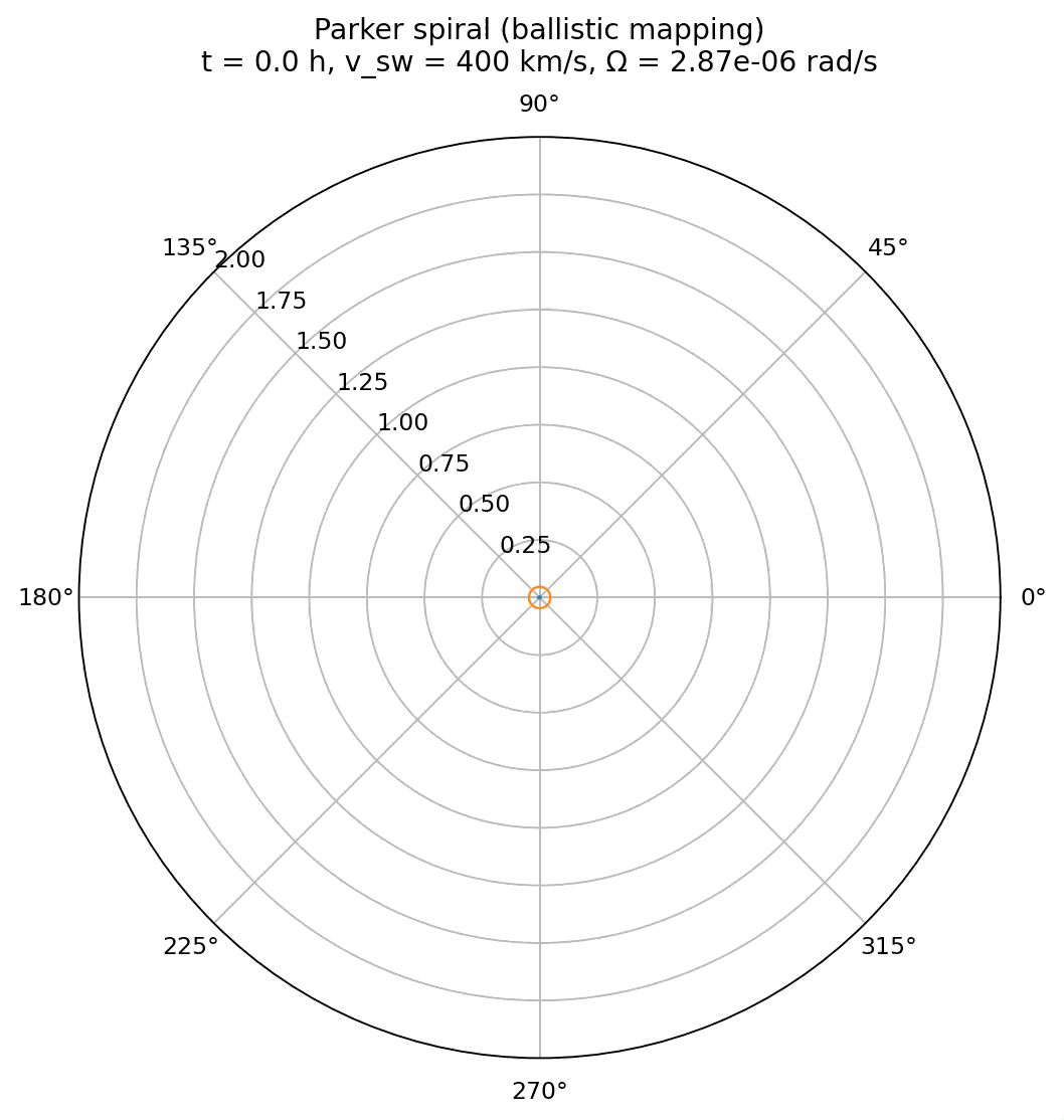
Simulation of the Parker spiral structure of the interplanetary magnetic field using ballistic mapping of radially propagating plasma parcels. The spiral is drawn for a solar wind speed of 400 km/s and a source surface at 10 solar radii.

The animation produced by the ballistic mapping code shows the Parker spiral emerging dynamically from the motion of individual plasma parcels. Unlike the analytical case, the spiral is not drawn as a predefined curve. Instead, it is reconstructed from the accumulated trajectories of many radially propagating plasma elements launched from a rotating source.

In this visualization, the spiral gradually builds up over time. Close to the source, newly launched parcels dominate the structure, while farther out, the spiral reflects the integrated launch history over many rotation periods. This makes explicit that magnetic field lines are not physical objects, but represent the instantaneous spatial organization of plasma elements whose motion is governed by flux freezing.

Relation to the analytical solution

Although this implementation is more elaborate than the analytical visualization, it does not introduce new physics. If the launch cadence is sufficiently fine and the domain large enough, the reconstructed spiral converges to the analytical Parker spiral derived earlier. The agreement between both approaches demonstrates that the spiral structure is not imposed by hand, but emerges naturally from the time dependent mapping between rotating footpoints and radially advected plasma.

This ballistic reconstruction therefore serves as an intermediate step between closed form theory and full magnetohydrodynamic simulations. It makes explicit how the Parker spiral arises from plasma motion, while still remaining transparent enough to be directly connected to the underlying analytical model.

Slow and fast solar wind speeds and their role in shaping the heliosphere

The Parker model itself does not prescribe a unique solar wind speed. Instead, the spiral geometry depends parametrically on the radial outflow velocity $v_{\mathrm{sw}}$. In the real heliosphere, the solar wind is not characterized by a single speed but by the coexistence of at least two distinct regimes: slow and fast solar wind. Understanding their origin and interaction is essential for interpreting the large-scale structure and dynamics of the heliosphere.

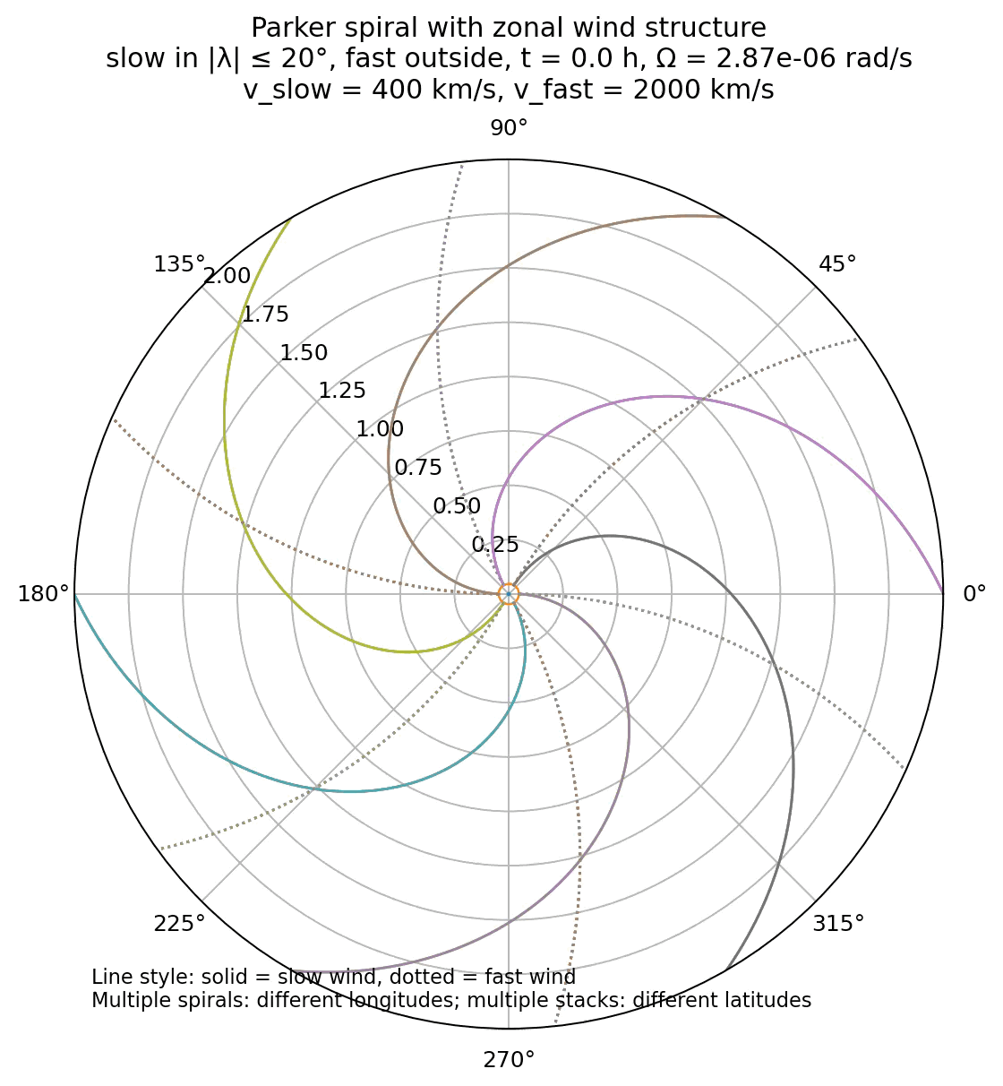
Another simulation result with parker spirals for both slow (400 km/s) and fast (2000 km/s) solar wind speeds. The code for generating this figure is not shown here, but available in the GitHub repository mentioned below

Physical origin of slow and fast solar wind

The fast solar wind typically exhibits speeds up to $2000\,\mathrm{km/s}$ and originates predominantly from coronal holes, regions of open magnetic field lines where plasma can escape efficiently. These regions are more common at higher heliographic latitudes during solar minimum, leading to a pronounced latitudinal structure of the solar wind.

The slow solar wind, with typical speeds around $300$ to $450\,\mathrm{km/s}$, is associated with the streamer belt and regions near the heliospheric current sheet. Its precise origin is more complex and remains an active research topic. Proposed mechanisms include plasma release from closed magnetic loops, interchange reconnection, and extended acceleration regions. Compared to the fast wind, the slow wind is generally denser, more variable, and exhibits stronger compositional signatures of coronal processing.

Consequences for Parker spiral geometry

In the Parker framework, the local orientation of the interplanetary magnetic field is determined by the ratio $\Omega r / v_{\mathrm{sw}}$. As a result, slow and fast solar wind naturally correspond to different spiral pitch angles. Slow wind produces a more tightly wound spiral, with a larger azimuthal magnetic field component, while fast wind leads to a more radially oriented field.

This dependence implies that there is no single, global Parker spiral geometry in the heliosphere. Instead, different magnetic flux tubes exhibit different spiral angles depending on the wind speed with which they are advected. Measurements at a fixed heliocentric distance therefore sample a distribution of Parker angles rather than a unique value, reflecting the structured nature of the solar wind.

Zonal structure and heliospheric dynamics

The coexistence of slow and fast wind gives rise to a zonal organization of the heliosphere, particularly evident during solar minimum. An equatorial band of slow wind is surrounded by faster wind at higher latitudes. This latitudinal variation produces a three-dimensional heliospheric structure in which magnetic field lines emerging from different source regions are wound to different degrees.

Importantly, these regions do not remain dynamically isolated. Fast solar wind streams originating at higher latitudes or from coronal holes can overtake slower wind emitted earlier along neighboring longitudes. When this occurs, the interaction does not result in a simple superposition of two Parker spirals. Instead, it leads to compression regions, enhanced magnetic field strengths, and shear flows. These structures are known as stream interaction regions, and when they persist over multiple solar rotations, as corotating interaction regions.

Such interaction regions play a central role in heliospheric dynamics. They modify the local magnetic field topology, contribute to turbulence generation, and are efficient sites for particle acceleration. Their existence highlights that the Parker spiral should be understood as a local, idealized description of individual flux tubes rather than as a globally static field configuration.

Implications for modeling and interpretation

From a modeling perspective, slow and fast solar wind speeds represent different realizations of the same underlying Parker mechanism rather than separate physical regimes. Each flux tube follows a Parker-type spiral determined by its effective outflow speed, but the collective heliosphere emerges from the spatial arrangement and interaction of many such flux tubes.

The zonal visualization presented here captures this idea in a simplified form:

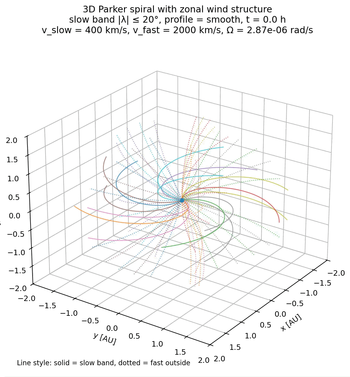
Simulation of the Parker spiral in 3D with both slow (400 km/s) and fast (2000 km/s) solar wind speeds assigned to different heliographic latitudes. The code for generating this figure is not shown here, but available in the GitHub repository mentioned below

By assigning different wind speeds to different heliographic latitudes, it illustrates how variations in $v_{\mathrm{sw}}$ alone are sufficient to produce a structured heliosphere with multiple spiral angles. At the same time, it makes clear what is missing: time dependence, stream interactions, and magnetic reconnection are essential for a complete description but lie beyond the scope of the Parker model.

In this sense, the distinction between slow and fast solar wind provides a bridge between the elegance of Parker’s analytical solution and the complexity observed in the real heliosphere. It shows how a simple theoretical framework can accommodate rich structure while also indicating where idealization must give way to full magnetohydrodynamic modeling.

Summary and discussion

The Parker model is intentionally simple. It neglects stream interactions, latitudinal structure, turbulence, and time dependent phenomena such as coronal mass ejections. Nevertheless, its core predictions remain foundational. The existence of a transonic solar wind and the spiral structure of the heliospheric magnetic field are direct consequences of basic conservation laws combined with solar rotation.

From a modern viewpoint, the Parker model should be understood not as a complete description of heliospheric plasma physics, but as the minimal theoretical framework upon which more sophisticated kinetic and magnetohydrodynamic models are built. Its lasting value lies precisely in this clarity: it shows that the solar wind and the Parker spiral are not exotic features, but unavoidable outcomes of a hot, rotating star embedded in a conducting plasma.

Update and code availability: This post and its accompanying Python code were originally drafted in 2020 and archived during the migration of this website to Jekyll and Markdown. In January 2026, I substantially revised and extended the code. The updated and cleaned-up implementation is now available in this new GitHub repositoryꜛ. Please feel free to experiment with it and to share any feedback or suggestions for further improvements.

References and further reading

Wolfgang Baumjohann and Rudolf A. Treumann, Basic Space Plasma Physics, 1997, Imperial College Press, ISBN: 1-86094-079-X
J. A. Bittencourt, Fundamentals of Plasma Physics, 2004, Springer, ISBN: 978-0-387-20975-3
Wikipedia article on the solar windꜛ