Magnetic reconnection: Theory and a simple numerical model

August 22, 2020 January 23, 2026 20 minute read see also comments

Magnetic reconnection denotes the process by which magnetic field lines in a conducting plasma change their topology, break, and reconnect. In doing so, magnetic energy stored in stressed field configurations is rapidly converted into bulk plasma motion, thermal energy, and non-thermal particle acceleration. Reconnection is therefore not a marginal effect but one of the central energy conversion mechanisms in plasma physics. It operates across an enormous range of scales, from laboratory fusion devices to planetary magnetospheres and the solar corona.

Animated schematic of magnetic reconnection. Animated are in- (top/bottom) and outflowing (left/right) plasma bundles. Source: Wikimedia Commonsꜛ (license: public domain).

In an ideal plasma with infinite electrical conductivity, magnetic field lines are frozen into the plasma flow and move together with it. This frozen-in condition breaks down when resistivity becomes finite or when strong gradients develop that invalidate the assumptions of ideal magnetohydrodynamics. At such locations, magnetic topology can change, enabling reconnection.

Physical picture

The basic reconnection geometry is conceptually simple. Two regions of oppositely directed magnetic field are driven together by plasma inflow. At their interface, a narrow diffusion region forms in which the frozen-in condition is violated. Field lines entering this region reconnect and form new connections. These newly connected field lines are strongly bent and relax outward, ejecting plasma in the form of high-speed jets along the outflow direction.

An artist’s concept depicts a flare evolving into a Coronal Mass Ejection (CME). Color-color diagrams may help scientists predict which flares will evolve into potentially dangerous Coronal Mass Ejections (CMEs), and which ones will fade back into the solar atmosphere. A CME is caused by a sudden reorganization of the Sun’s magnetic field, i.e., magnetic reconnection. Source: Wikimedia Commonsꜛ (license: public domain).

This process naturally explains why reconnection is both localized and explosive. Energy is stored globally in large-scale magnetic fields but released locally in thin current sheets. Once reconnection sets in, magnetic tension accelerates plasma to speeds comparable to the Alfvén velocity, and the system rapidly transitions to a lower-energy magnetic configuration.

MHD formulation

Within resistive magnetohydrodynamics, magnetic reconnection follows directly from the induction equation

\[\begin{align} \frac{\partial \mathbf{B}}{\partial t} = \nabla \times (\mathbf{v} \times \mathbf{B}) \nabla \times (\eta \nabla \times \mathbf{B}), \end{align}\]

where $\mathbf{B}$ is the magnetic field, $\mathbf{v}$ the plasma velocity, and $\eta$ the electrical resistivity.

In the limit $\eta \to 0$, the diffusive term vanishes and magnetic flux is conserved, enforcing the frozen-in condition. Reconnection becomes possible only in regions where the resistive term competes with the inductive term, typically inside thin current sheets where $\nabla \times \mathbf{B}$ becomes large.

The energetic aspect of reconnection follows from the Poynting theorem. The local rate of magnetic energy conversion is governed by the work done by the electric field on the current,

\[\begin{align} -\mathbf{E} \cdot \mathbf{J}, \end{align}\]

which directly transfers electromagnetic energy into particle motion and heat.

The Sweet–Parker model

The first quantitative model of reconnection was developed independently by Peter Sweet and Eugene Parker in the late 1950s. In the Sweet–Parker framework, reconnection occurs in an elongated diffusion region of length $L$ and thickness $\delta$.

Plasma carrying magnetic field lines flows into the sheet with velocity $v_{\text{in}}$ and exits along the sheet with velocity close to the Alfvén speed.

\[\begin{align} v_A = \frac{B}{\sqrt{\mu_0 \rho}}, \end{align}\]

where $\rho$ is the mass density. Mass and flux conservation imply

\[\begin{align} v_{\text{in}} , \delta \approx v_A , L. \end{align}\]

Balancing advection and diffusion across the sheet yields a reconnection inflow speed

$\begin{align} v_{\text{in}} \approx \frac{v_A}{\sqrt{S}}, \end{align}$ where

\[\begin{align} S = \frac{\mu_0 L v_A}{\eta} \end{align}\]

is the Lundquist number. For astrophysical plasmas, $S$ is typically enormous, often exceeding $10^{12}$. As a consequence, the Sweet–Parker reconnection rate is far too slow to account for rapid phenomena such as solar flares.

The Petschek model

A major conceptual advance was proposed by Harry Petschek, who suggested that fast reconnection is possible if the diffusion region is short and the energy conversion is mediated by standing slow-mode shocks extending away from it.

In the Petschek scenario, the inflow speed scales as

\[\begin{align} v_{\text{in}} \approx \frac{\pi}{8 \ln S} , v_A, \end{align}\]

which depends only logarithmically on the Lundquist number. This allows reconnection rates compatible with solar and magnetospheric observations. While later numerical work has shown that achieving Petschek-like configurations requires additional physics beyond uniform resistive MHD, the model remains conceptually important for understanding fast reconnection.

Dimensionless control parameters

Several dimensionless numbers characterize reconnection regimes. The reconnection rate is often expressed as

\[\begin{align} M = \frac{v_{\text{in}}}{v_A}. \end{align}\]

The magnetic Reynolds number

\[\begin{align} R_m = \frac{\mu_0 v L}{\eta} \end{align}\]

measures the relative importance of advection and diffusion of magnetic fields. Large $R_m$ corresponds to frozen-in behavior on global scales, while reconnection becomes possible locally where effective diffusion is enhanced.

Energy conversion and particle acceleration

In the diffusion region, Ohm’s law reduces approximately to

\[\begin{align} \mathbf{E} \approx \eta \mathbf{J}, \end{align}\]

so that the power dissipated is

\[\begin{align} P = \int_V \mathbf{E} \cdot \mathbf{J} , dV. \end{align}\]

This leads to Joule heating of the plasma. In many space plasmas, however, collisionless effects dominate and additional mechanisms such as Hall currents, pressure tensor effects, and wave–particle interactions enable efficient particle acceleration far beyond what classical resistivity would predict.

Reconnection in natural and laboratory plasmas

Magnetic reconnection is directly observed and inferred in many environments. At Earth, reconnection on the dayside magnetopause couples the interplanetary magnetic field to the terrestrial field, enabling solar wind energy transfer. In the magnetotail, reconnection drives substorms and auroral activity.

Simulation of Earth’s magnetic field in interaction with (solar) interplanetar magnetic field (IMF): The animation illustrates the dynamical changes of the global magnetic field in the course of a disturbance: A temporary compression of the magnetosphere by enhanced flow of the solar wind is followed by a tailward stretching of the field lines. Eventually, the increase of the tail magnetic field results in a sudden collapse of the nightside field (a substorm) and a gradual recovery of the magnetosphere to its pre-storm configuration. Reconnections in the tail region (right) are only indicated as a preliminary stage. Source: Wikimedia Commonsꜛ (license: public domain).

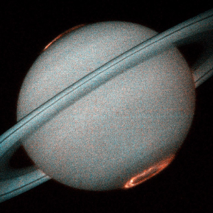
In the solar corona, reconnection is widely regarded as the central mechanism behind solar flares and coronal mass ejections, where vast amounts of magnetic energy are released on short timescales. In the magnetospheres of Jupiter and Saturn, reconnection in the magnetotail leads to the formation and release of plasmoids, producing quasi-periodic energy outbursts.

In laboratory plasmas, reconnection occurs in tokamaks and stellarators, where it can trigger sawtooth crashes and other instabilities that limit confinement.

Significance and broader implications

Magnetic reconnection provides a unifying explanation for explosive energy release in plasmas. It governs the coupling between stellar winds and planetary magnetospheres, drives space weather phenomena that affect technological systems, and poses fundamental challenges for controlled nuclear fusion. From a theoretical perspective, it represents a paradigmatic example of how small-scale non-ideal effects control large-scale plasma dynamics.

In my view, reconnection is also conceptually important because it exposes the limits of idealized descriptions. It demonstrates how global plasma behavior can hinge on localized breakdowns of otherwise robust conservation laws. For space plasma physics in particular, reconnection is not a special process at isolated sites, but a persistent and organizing principle of magnetized plasma systems.

Numerical modeling of reconnection

To illustrate the basic geometry and dynamics of magnetic reconnection, we deploy a deliberately simplified two-dimensional numerical model. The aim of this model is not quantitative realism, but conceptual clarity: it reproduces the canonical inflow–outflow structure of reconnection, the formation of a current sheet, and the topological change of magnetic field lines in a controlled and transparent setting.

Governing equations

The magnetic field is represented via an out-of-plane vector potential $(A(x,y,t))$, such that

\[\begin{align} B_x = \frac{\partial A}{\partial y}, \qquad B_y = -\frac{\partial A}{\partial x}. \end{align}\]

In this formulation, magnetic field lines correspond exactly to contour lines of $(A)$, which makes changes in magnetic topology directly visible.

The temporal evolution of $(A)$ is governed by a kinematic resistive magnetohydrodynamic equation,

\[\begin{align} \frac{\partial A}{\partial t} + \mathbf{v}\cdot\nabla A = \nabla\cdot\left(\eta \nabla A\right), \end{align}\]

where $\mathbf{v}(x,y)$ is a prescribed velocity field and $\eta(x,y)$ is a spatially varying resistivity. Importantly, the velocity field is not evolved self-consistently from the MHD momentum equation. Instead, it is imposed externally, allowing the reconnection geometry to be controlled explicitly.

Initial magnetic configuration

The initial magnetic field is based on a Harris-type current sheet, featuring antiparallel magnetic fields across $(y=0)$. In terms of the vector potential, this corresponds to

\[\begin{align} A_{\mathrm{Harris}}(y) = B_0 \, \delta_{\mathrm{cs}} \, \ln\cosh\left(\frac{y}{\delta_{\mathrm{cs}}}\right), \end{align}\]

which produces a smooth reversal of $(B_x)$ across a current sheet of half-thickness $(\delta_{\mathrm{cs}})$.

To trigger reconnection, a small, localized perturbation is added near the origin. This perturbation seeds an X-point in the magnetic topology and breaks the translational symmetry of the current sheet, allowing reconnection to develop dynamically.

Prescribed flow field

The inflow–outflow pattern characteristic of magnetic reconnection is imposed through a localized stagnation-point flow,

\[\begin{align} \mathbf{v}(x,y) = \bigl(+\alpha x,-\alpha y\bigr) \exp\left[-\frac{x^2+y^2}{w_v^2}\right]. \end{align}\]

This velocity field drives plasma toward the current sheet from above and below, while expelling plasma along the sheet in the $(\pm x)$ directions. The Gaussian envelope confines the flow to the central region of the domain, ensuring that reconnection remains localized and that boundary effects are minimized.

Because the flow is prescribed, the model isolates the role of advection and diffusion in the induction equation without introducing additional nonlinearities from momentum balance or pressure gradients.

Localized resistivity and diffusion region

Reconnection is enabled through a spatially localized enhancement of resistivity,

\[\begin{align} \eta(x,y) = \eta_{\mathrm{bg}} + \eta_{\mathrm{peak}} \exp\left[-\frac{x^2+y^2}{w_\eta^2}\right]. \end{align}\]

Outside the central diffusion region, the resistivity is small, approximating ideal MHD behavior and flux freezing. Near the origin, resistive diffusion becomes significant, allowing magnetic field lines to break and reconnect. This separation of ideal and non-ideal regions mirrors the conceptual structure of classical Sweet–Parker reconnection, albeit without enforcing its steady-state scaling relations.

Numerical implementation and visualization

The induction equation is discretized on a uniform Cartesian grid using second-order finite differences. Periodic boundary conditions are applied in the $(x)$ direction, while zero-gradient (Neumann) conditions are used in $(y)$. Time integration is performed explicitly using a forward Euler scheme with a timestep constrained by both advective and diffusive stability criteria.

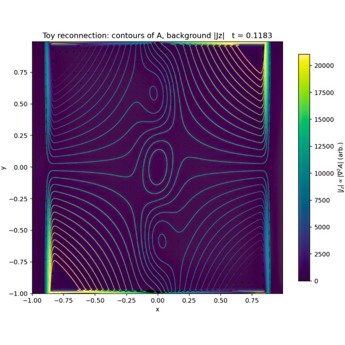
Magnetic reconnection is visualized by plotting contours of the vector potential $(A)$, which represent magnetic field lines exactly in two dimensions. The current density $(J_z \propto -\nabla^2 A)$ is shown as a background color map, highlighting the formation and evolution of the current sheet and diffusion region. A simple diagnostic of reconnection activity is obtained by evaluating the reconnection electric field $(E_z = \eta J_z)$ at the X-point.

Scope and limitations

This model is intentionally kinematic and resistive. It neglects momentum balance, pressure, compressibility, Hall physics, and kinetic effects. As a result, it does not aim to reproduce reconnection rates, plasmoid statistics, or energetic particle acceleration quantitatively. Instead, it provides a minimal, transparent framework that captures the essential geometry of magnetic reconnection and the interplay between advection, diffusion, and topology change.

In this sense, the model should be read as a numerical analogue of a textbook reconnection diagram: dynamically consistent, physically motivated, but optimized for insight rather than realism.

Python code

We begin by importing the necessary libraries:

from __future__ import annotations

from pathlib import Path
import numpy as np
import matplotlib.pyplot as plt
import imageio.v2 as imageio

Next, we define several helper functions for our simulation. In the following, we define functions for

ensuring the output directory exists,
finite difference operators with mixed boundary conditions,
computing magnetic field and current density from the vector potential, and
setting up initial conditions for the vector potential.

# function to ensure output directory exists:
def ensure_dir(p: str | Path) -> None:
    Path(p).mkdir(parents=True, exist_ok=True)

# functions for finite differences with various BCs:
def ddx_periodic(f: np.ndarray, dx: float) -> np.ndarray:
    return (np.roll(f, -1, axis=1) - np.roll(f, 1, axis=1)) / (2.0 * dx)

# function for finite differences with various BCs:
def ddy_neumann(f: np.ndarray, dy: float) -> np.ndarray:
    """
    Central difference in y with zero-gradient (Neumann) boundary.
    Implemented by edge padding.
    """
    fp = np.pad(f, ((1, 1), (0, 0)), mode="edge")
    return (fp[2:, :] - fp[:-2, :]) / (2.0 * dy)

# function for finite differences with various BCs:
def laplacian_mixed(f: np.ndarray, dx: float, dy: float) -> np.ndarray:
    """
    Laplacian: periodic in x, Neumann (zero-gradient) in y.
    """
    f_xx = (np.roll(f, -1, axis=1) - 2.0 * f + np.roll(f, 1, axis=1)) / (dx * dx)

    fp = np.pad(f, ((1, 1), (0, 0)), mode="edge")
    f_yy = (fp[2:, :] - 2.0 * fp[1:-1, :] + fp[:-2, :]) / (dy * dy)

    return f_xx + f_yy

# function for finite differences with various BCs:
def grad_eta_dot_grad_A(eta: np.ndarray, A: np.ndarray, dx: float, dy: float) -> np.ndarray:
    """
    Compute ∇·(η ∇A) = η ∇²A + (∇η)·(∇A), with mixed BCs.
    """
    lapA = laplacian_mixed(A, dx, dy)
    etax = ddx_periodic(eta, dx)
    etay = ddy_neumann(eta, dy)
    Ax = ddx_periodic(A, dx)
    Ay = ddy_neumann(A, dy)
    return eta * lapA + (etax * Ax + etay * Ay)

# function to compute B and Jz from A:
def compute_B(A: np.ndarray, dx: float, dy: float) -> tuple[np.ndarray, np.ndarray]:
    Bx = ddy_neumann(A, dy)
    By = -ddx_periodic(A, dx)
    return Bx, By

# function to compute Jz from A:
def compute_Jz(A: np.ndarray, dx: float, dy: float) -> np.ndarray:
    # Jz ∝ (∇×B)_z = -∇²A in these conventions
    return -laplacian_mixed(A, dx, dy)

Then, we define functions for setting up the initial conditions of the simulation:

# function to make initial A:
def A_harris(Y: np.ndarray, B0: float, delta_cs: float) -> np.ndarray:
    """
    Harris sheet: Bx(y) = B0 tanh(y/delta_cs)
    A(y) = B0 * delta_cs * ln cosh(y/delta_cs)
    """
    return B0 * delta_cs * np.log(np.cosh(Y / delta_cs) + 1e-30)

# function to make initial A perturbation:
def A_perturbation(X: np.ndarray, Y: np.ndarray, a: float, kx: float, sigma_y: float) -> np.ndarray:
    """
    Localized perturbation that seeds an X-point around (0,0).
    """
    return a * np.cos(kx * X) * np.exp(-(Y * Y) / (2.0 * sigma_y * sigma_y))

and we define the main plotting function for visualizing the simulation results:

def plot_frame(A: np.ndarray,
                       vx: np.ndarray,
                       vy: np.ndarray,
                       X: np.ndarray,
                       Y: np.ndarray,
                       dx: float,
                       dy: float,
                       t: float,
                       out_png: str,
                       diff_box: float = 0.12,
                       streamline_density: float = 1.2,
                       show_velocity: bool = False) -> None:
    Bx, By = compute_B(A, dx, dy)
    Jz = compute_Jz(A, dx, dy)
    Jabs = np.abs(Jz)
    vmaxJ = np.percentile(Jabs, 99.7) + 1e-12

    fig = plt.figure(figsize=(8.2, 5.6), dpi=150)
    ax = fig.add_subplot(1, 1, 1)

    im = ax.imshow(
        Jabs,
        origin="lower",
        extent=[X.min(), X.max(), Y.min(), Y.max()],
        aspect="auto",
        vmin=0.0,
        vmax=vmaxJ,
        interpolation="bilinear")
    cb = fig.colorbar(im, ax=ax, shrink=0.9)
    cb.set_label(r"$|J_z| \propto |\nabla^2 A|$ (arb.)")

    # streamlines: top (red) and bottom (blue)
    # choose start points in two horizontal lines above and below the sheet
    nseed = 20
    xs = np.linspace(X.min() * 0.95, X.max() * 0.95, nseed)

    y_top = 0.65 * Y.max()
    y_bot = 0.65 * Y.min()

    start_top = np.column_stack([xs, np.full_like(xs, y_top)])
    start_bot = np.column_stack([xs, np.full_like(xs, y_bot)])

    # draw separately to enforce color:
    levels = np.linspace(np.percentile(A, 5), np.percentile(A, 95), 18)

    A_top = np.where(Y >= 0, A, np.nan)
    A_bot = np.where(Y <= 0, A, np.nan)

    ax.contour(X, Y, A_top, levels=levels, colors="red", linewidths=2.2)
    ax.contour(X, Y, A_bot, levels=levels, colors="blue", linewidths=2.2)
    
    
    # diffusion region box:
    from matplotlib.patches import Rectangle
    rect = Rectangle((-diff_box, -diff_box), 2.0 * diff_box, 2.0 * diff_box,
                     fill=False, lw=2.0, edgecolor="gold")
    ax.add_patch(rect)

    # schematic inflow/outflow arrows:
    # inflow: from top and bottom towards origin
    ax.annotate("", xy=(0.0, 0.22), xytext=(0.0, 0.60),
                arrowprops=dict(arrowstyle="simple", color="gold", alpha=0.5))
    ax.annotate("", xy=(0.0, -0.22), xytext=(0.0, -0.60),
                arrowprops=dict(arrowstyle="simple", color="gold", alpha=0.5))

    # outflow: from origin to left/right:
    ax.annotate("", xy=(0.60, 0.0), xytext=(0.22, 0.0),
                arrowprops=dict(arrowstyle="simple", color="gold", alpha=0.5))
    ax.annotate("", xy=(-0.60, 0.0), xytext=(-0.22, 0.0),
                arrowprops=dict(arrowstyle="simple", color="gold", alpha=0.5))

    # optional velocity quiver (subsampled):
    if show_velocity:
        stride = 14
        ax.quiver(X[::stride, ::stride], Y[::stride, ::stride],
                  vx[::stride, ::stride], vy[::stride, ::stride],
                  angles="xy", scale_units="xy", scale=None, width=0.0022, alpha=0.35, color="k")

    ax.set_title(f"2D reconnection simulation (toy model)   t = {t:.4f}")
    ax.set_xlabel("x")
    ax.set_ylabel("y")
    ax.set_xlim(X.min(), X.max())
    ax.set_ylim(Y.min(), Y.max())

    fig.tight_layout()
    fig.savefig(out_png)
    plt.close(fig)

Last, we construct the main simulation function that ties everything together:

def run_reconnection_simulation(out_dir: str = "reconnection_out",
                             nx: int = 420,
                             ny: int = 260,
                             Lx: float = 2.0,
                             Ly: float = 2.0,
                             B0: float = 1.0,
                             delta_cs: float = 0.08,
                             a_pert: float = 0.06,
                             sigma_y: float = 0.20,
                             alpha: float = 1.2,
                             w_v: float = 0.65,
                             eta_bg: float = 8e-4,
                             eta_peak: float = 8e-3,
                             w_eta: float = 0.14,
                             t_end: float = 1.0,
                             cfl_adv: float = 0.35,
                             cfl_diff: float = 0.20,
                             frame_every: int = 1,
                             gif_fps: int = 28,
                             show_velocity: bool = False) -> None:
    out_path = Path(out_dir)
    frames_dir = out_path / "frames"
    ensure_dir(frames_dir)
    ensure_dir(out_path)

    # grid
    x = np.linspace(-Lx / 2.0, Lx / 2.0, nx, endpoint=False)
    y = np.linspace(-Ly / 2.0, Ly / 2.0, ny, endpoint=True)
    dx = x[1] - x[0]
    dy = y[1] - y[0]
    X, Y = np.meshgrid(x, y)

    # prescribed inflow/outflow flow: inflow in y, outflow in x:
    phi_v = np.exp(-(X * X + Y * Y) / (w_v * w_v))
    vx = (+alpha * X) * phi_v
    vy = (-alpha * Y) * phi_v

    # resistivity profile: background + localized enhancement (diffusion region):
    eta = eta_bg + eta_peak * np.exp(-(X * X + Y * Y) / (w_eta * w_eta))

    # initial A: Harris sheet + perturbation
    kx = 2.0 * np.pi / Lx
    A = A_harris(Y, B0=B0, delta_cs=delta_cs) + A_perturbation(X, Y, a=a_pert, kx=kx, sigma_y=sigma_y)

    # stable dt (explicit):
    vmax = max(np.max(np.abs(vx)), np.max(np.abs(vy)))
    if vmax == 0.0:
        dt_adv = np.inf
    else:
        dt_adv = cfl_adv * min(dx, dy) / (vmax + 1e-30)

    # diffusion stability uses max(eta):
    eta_max = float(np.max(eta))
    dt_diff = cfl_diff * min(dx * dx, dy * dy) / (eta_max + 1e-30)
    dt = min(dt_adv, dt_diff)

    n_steps = int(np.ceil(t_end / dt))
    mid_step = n_steps // 2

    initial_png = out_path / "initial.png"
    middle_png = out_path / "middle.png"
    final_png = out_path / "final.png"

    frame_paths: list[Path] = []

    def save_frame(step: int, t_now: float) -> None:
        fn = frames_dir / f"frame_{step:06d}.png"
        plot_frame(A, vx, vy, X, Y, dx, dy, t_now, str(fn),
                           diff_box=0.12, streamline_density=1.15,
                           show_velocity=show_velocity)
        frame_paths.append(fn)

    # initial snapshot + frame 0:
    t = 0.0
    plot_frame(A, vx, vy, X, Y, dx, dy, t, str(initial_png),
                       diff_box=0.12, streamline_density=1.15,
                       show_velocity=show_velocity)
    if frame_every == 1:
        save_frame(0, t)

    # time stepping:
    for step in range(1, n_steps + 1):
        if t + dt > t_end:
            dt = t_end - t

        # advection terms:
        Ax = ddx_periodic(A, dx)
        Ay = ddy_neumann(A, dy)

        adv = -(vx * Ax + vy * Ay)

        # diffusion term with spatially varying eta:
        diff = grad_eta_dot_grad_A(eta, A, dx, dy)

        # explicit Euler update:
        A = A + dt * (adv + diff)
        t += dt

        if step == mid_step:
            plot_frame(A, vx, vy, X, Y, dx, dy, t, str(middle_png),
                               diff_box=0.12, streamline_density=1.15,
                               show_velocity=show_velocity)

        if step % frame_every == 0:
            save_frame(step, t)
            
        # reconnection diagnostic at X-point:
        if step % 100 == 0:
            iy, ix = np.unravel_index(np.argmin(X**2 + Y**2), X.shape)
            Ez = eta[iy, ix] * compute_Jz(A, dx, dy)[iy, ix]
            print(f"step={step}, t={t:.3f}, Ez={Ez:.3e}")

    # final snapshot:
    plot_frame(A, vx, vy, X, Y, dx, dy, t, str(final_png),
                       diff_box=0.12, streamline_density=1.15,
                       show_velocity=show_velocity)

    # build gif:
    gif_path = out_path / "reconnection.gif"
    images = [imageio.imread(p) for p in frame_paths]
    imageio.mimsave(gif_path, images, fps=gif_fps)

    print("Done.")
    print(f"Output directory: {out_path.resolve()}")
    print(f"GIF: {gif_path.resolve()}")
    print(f"Initial: {initial_png.resolve()}")
    print(f"Middle: {middle_png.resolve()}")
    print(f"Final: {final_png.resolve()}")
    print(f"Frames: {frames_dir.resolve()} (count: {len(frame_paths)})")
    print(f"dt used ~ {t_end / max(n_steps,1):.3e}  steps: {n_steps}")

Finally, we call the main simulation function with specific parameters to run the reconnection simulation and generate output visualizations:

run_reconnection_simulation(
        out_dir="reconnection_out", # defined output directory
        nx=420,                     # resolution: grid points in x
        ny=260,                     # resolution: grid points in y
        Lx=2.0,                     # box size in x (box defines the central region)
        Ly=2.0,                     # box size in y
        B0=1.0,                     # asymptotic magnetic field strength
        delta_cs=0.08,              # current sheet half-thickness
        a_pert=0.20,                # perturbation amplitude; use values between 0.06 and 0.20; higher values lead to faster reconnection onset
        sigma_y=0.08,               # perturbation width in y; smaller values lead to faster reconnection onset
        alpha=1.4,                  # inflow/outflow strength
        w_v=0.65,                   # inflow/outflow width scale
        eta_bg=8e-4,                # background resistivity
        eta_peak=8.0e-2, # or 8e-3  # peak resistivity in diffusion region
        w_eta=0.05,      # or 0.14  # resistivity enhancement width scale
        t_end=4.0,       # or 3.0   # end time of simulation
        frame_every=100,            # save every N steps; the higher the faster the simulation
        gif_fps=28,                 # fps for the output gif
        show_velocity=False,        # whether to show velocity quiver
    )

Discussion

The numerical model presented here is intentionally minimal and kinematic in nature. It evolves the out-of-plane vector potential $A(x,y,t)$ according to a resistive induction equation with a prescribed velocity field and spatially localized resistivity. As a result, the magnetic field topology evolves self-consistently through advection and diffusion of magnetic flux, while the plasma flow itself is not influenced by the magnetic field. This separation makes the model particularly suitable for didactic purposes, as it cleanly isolates the geometrical and topological aspects of magnetic reconnection from the full dynamical complexity of magnetohydrodynamics.

Time evolution of our two-dimensional magnetic reconnection toy model based on the resistive induction equation for the magnetic flux function $A(x,y,t)$. Magnetic field lines (contours of $A$) are shown in red (upper half-plane) and blue (lower half-plane), while the background color indicates the magnitude of the out-of-plane current density $|J_z| \propto |\nabla^2 A|$. A Harris-type current sheet at $y=0$ is perturbed to seed an X-point, and a prescribed stagnation flow drives plasma inflow from top and bottom and outflow to the left and right. A localized resistivity enhancement marks the diffusion region (yellow box). The sequence illustrates thinning of the current sheet, formation of a localized reconnection region, and the expulsion of reconnected flux into outflow jets. Shown are the initial state, an intermediate stage, and the final configuration of the simulation.

Starting from a Harris-like current sheet with anti-parallel magnetic fields across $y=0$, a localized perturbation introduces an X-point at the center of the domain. The imposed stagnation flow continuously advects magnetic flux toward the current sheet from above and below, while newly reconnected field lines are expelled horizontally. In combination with a localized enhancement of the resistivity, this setup reproduces the essential ingredients of classical two-dimensional reconnection models: flux pile-up, current sheet thinning, localized breaking of field line connectivity, and the formation of reconnection outflows.

The animation demonstrates several qualitative features that are central to reconnection physics. First, magnetic flux is transported into the diffusion region by advection rather than being created or destroyed globally. Second, reconnection remains spatially localized despite the extended current sheet, emphasizing the role of enhanced dissipation in enabling topological change. Third, the post-reconnection field lines are rapidly swept away from the X-point, preventing an unphysical accumulation of reconnected flux and maintaining a quasi-steady reconnection geometry.

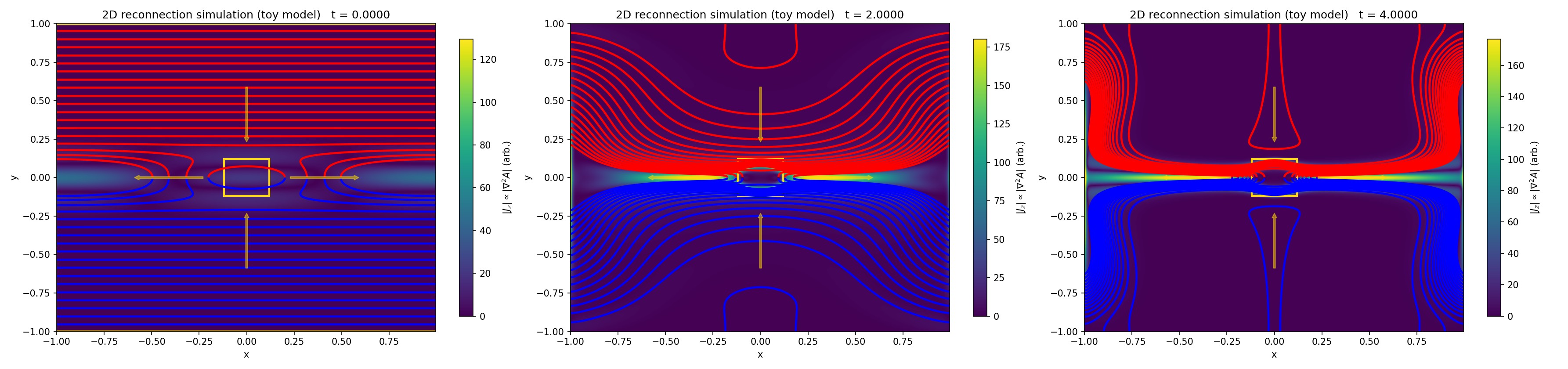
Initial (left), intermediate (center), and final (right) states of the two-dimensional magnetic reconnection toy model.

At the same time, it is important to stress the limitations of the model. Because the velocity field is prescribed and incompressible, there is no momentum balance, no feedback of magnetic tension on the flow, and no self-consistent formation of outflow jets or shocks. Effects such as plasmoid instability, Hall physics, guide fields, pressure anisotropy, and kinetic scale processes are entirely absent. Consequently, the model should not be interpreted quantitatively or compared directly to laboratory, space, or astrophysical reconnection rates. Instead, it provides an intuitive illustration of how magnetic reconnection reorganizes field topology under the combined action of advection and localized resistive diffusion.

Feel free to download and run the provided Python code to explore the parameter space and visualize different reconnection scenarios. Adjusting parameters such as the perturbation amplitude, resistivity profile, and inflow strength can yield a variety of reconnection dynamics, all within the conceptual framework outlined above.

Stay tuned for a follow-up post, where I discuss a complementary toy model based on X-point collapse and highlight how different geometries and driving assumptions shape the reconnection dynamics.

Update and code availability: This post and its accompanying Python code were originally drafted in 2020 and archived during the migration of this website to Jekyll and Markdown. In January 2026, I substantially revised and extended the code. The updated and cleaned-up implementation is now available in this new GitHub repositoryꜛ. Please feel free to experiment with it and to share any feedback or suggestions for further improvements.

References and further reading

Wolfgang Baumjohann and Rudolf A. Treumann, Basic Space Plasma Physics, 1997, Imperial College Press, ISBN: 1-86094-079-X
J. A. Bittencourt, Fundamentals of Plasma Physics, 2004, Springer, ISBN: 978-0-387-20975-3
Wikipedia article on Magnetic Reconnectionꜛ