The Alfvén wave as a fundamental mode of magnetized plasmas

Among all plasma waves, the Alfvén wave occupies a special conceptual position. It is the simplest genuinely magnetized plasma mode, arising directly from the coupling between magnetic field line tension and plasma inertia. At the same time, it provides a concrete and analytically tractable example of how collective plasma dynamics interpolate between fluid and kinetic descriptions. In space plasmas, Alfvén waves dominate large scale fluctuations in the solar wind, control energy transport along magnetic field lines, and form the backbone of magnetosphere ionosphere coupling.

Magnetohydrodynamic shear Alfvén wave linear perturbations. Alfvén waves are transverse, incompressible oscillations of magnetic field lines in a magnetized plasma. The background magnetic field $\mathbf{B}_0$ provides tension that acts as the restoring force, while the bulk plasma mass density $\rho_0$ (not shown here) provides inertia. Perturbations in the velocity $\mathbf{v}_1$ and magnetic field $\mathbf{B}_1$ are perpendicular to both the background field and the wave vector $\mathbf{k}$. The total magnetic field is $\mathbf {B} =\mathbf {B}_{0}+\mathbf {B}_{1}$. Source: Wikimedia Commonsꜛ (license: CC BY-SA 4.0).

Mathematically, the Alfvén wave emerges already in ideal magnetohydrodynamics as a transverse, incompressible mode propagating along the background magnetic field. Yet this apparently simple wave admits a hierarchy of increasingly refined descriptions, from ideal MHD to Hall MHD and fully kinetic theory. The Alfvén wave therefore serves as a natural entry point for understanding magnetized linear plasma oscillations.

In this post, we derive the Alfvén wave from first principles, explore its fundamental properties, and discuss its physical interpretation.

Linearized magnetohydrodynamics

The starting point is the system of ideal magnetohydrodynamics, describing a perfectly conducting plasma treated as a single fluid. The governing equations are the continuity equation, the momentum equation, the induction equation, and an equation of state. Written explicitly,

\[\begin{aligned} \partial_t \rho + \nabla\cdot(\rho \mathbf{u}) &= 0, \\ \rho\left(\partial_t \mathbf{u} + \mathbf{u}\cdot\nabla\mathbf{u}\right) &= -\nabla p + \frac{1}{\mu_0}(\nabla\times\mathbf{B})\times\mathbf{B},\\ \partial_t \mathbf{B} &= \nabla\times(\mathbf{u}\times\mathbf{B}), \end{aligned}\]

supplemented by $\nabla\cdot\mathbf{B}=0$ and a closure relating pressure and density.

We linearize around a homogeneous equilibrium with constant density $\rho_0$, pressure $p_0$, and a uniform background magnetic field $\mathbf{B}_0$. Perturbations are denoted by $\rho_1$, $\mathbf{u}_1$, $\mathbf{B}_1$, and $p_1$, assumed small compared to the background quantities. Keeping only first order terms yields the linearized system.

Incompressible limit and transverse dynamics

The Alfvén wave appears most transparently in the incompressible limit, where density and pressure perturbations are neglected and $\nabla\cdot\mathbf{u}_1 = 0$. The linearized momentum equation reduces to

\[\rho_0 \partial_t \mathbf{u}_1 = \frac{1}{\mu_0}(\nabla\times\mathbf{B}_1)\times\mathbf{B}_0.\]

The induction equation becomes

\[\partial_t \mathbf{B}_1 = \nabla\times(\mathbf{u}_1\times\mathbf{B}_0).\]

Assuming plane wave solutions of the form $\exp[i(\mathbf{k}\cdot\mathbf{x}-\omega t)]$ and choosing $\mathbf{k}$ with a component parallel to $\mathbf{B}_0$, one finds that solutions exist with perturbations perpendicular to both $\mathbf{k}$ and $\mathbf{B}_0$. These are shear Alfvén waves.

Dispersion relation and Alfvén speed

Combining the linearized momentum and induction equations yields a wave equation for the transverse velocity perturbation,

\[\partial_t^2 \mathbf{u}_{1\perp} = v_A^2 \,\partial_\parallel^2 \mathbf{u}_{1\perp},\]

where

• $\mathbf{u}_{1\perp}$ denotes the velocity perturbation perpendicular to the background magnetic field $\mathbf{B}_0$, and
• $\partial_{\parallel} = \hat{\mathbf{b}}\cdot\nabla$ is the derivative along the field direction $\hat{\mathbf{b}}=\mathbf{B}_0 / \lVert \mathbf{B}_0 \rVert$.

The constant

\[v_A = \frac{B_0}{\sqrt{\mu_0 \rho_0}}\]

is the Alfvén speed, set by the background magnetic field strength $B_0$ and the plasma mass density $\rho_0$.

For plane wave solutions of the form $\exp[i(\mathbf{k}\cdot\mathbf{x}-\omega t)]$, the corresponding dispersion relation is

\[\omega = k_\parallel v_A,\]

with $k_\parallel=\mathbf{k}\cdot\hat{\mathbf{b}}$.

Several key features follow immediately. The wave propagates strictly along magnetic field lines. It is nondispersive in ideal MHD, meaning that phase and group velocity coincide. The restoring force is magnetic tension, while inertia is provided by the bulk plasma mass density.

Polarization and physical interpretation

In an Alfvén wave, both the velocity perturbation $\mathbf{u}_1$ and the magnetic field perturbation $\mathbf{B}_1$ are transverse to the background field $\mathbf{B}_0$. Their amplitudes are related by

\[\mathbf{B}_1 = \pm \sqrt{\mu_0 \rho_0}\,\mathbf{u}_1,\]

where the sign is determined by the propagation direction relative to $\mathbf{B}_0$. This relation reflects the fact that Alfvén waves correspond to transverse oscillations of magnetic field lines, with the plasma frozen into the field.

From an energy perspective, Alfvén waves continuously exchange kinetic energy of the plasma flow with magnetic energy stored in bent field lines. This exchange is lossless in ideal MHD.

Relation to magnetosonic modes

Alfvén waves form one branch of the three fundamental MHD wave modes. Including compressibility but retaining ideal MHD, the Alfvén branch satisfies

\[\omega^2 = k^2 v_A^2 \cos^2\theta,\]

where $\theta$ is the angle between the wave vector $\mathbf{k}$ and the background magnetic field $\mathbf{B}_0$. The remaining solutions correspond to the fast and slow magnetosonic modes, which involve compressive density and pressure fluctuations. The Alfvén wave is distinguished by the absence of density and pressure fluctuations, which makes it robust in low beta plasmas and dominant in many space environments.

Group velocity and energy transport

Because the dispersion relation is linear in $k_\parallel$, the group velocity is given by

\[\mathbf{v}_g = \nabla_{\mathbf{k}}\omega = v_A\,\hat{\mathbf{b}},\]

directed strictly along the background magnetic field, where $\hat{\mathbf{b}}$ is the unit vector along the background magnetic field. Energy therefore propagates strictly along field lines. This property underlies the role of Alfvén waves as carriers of electromagnetic energy between distant regions of a magnetized plasma, for example between the magnetosphere and ionosphere.

The associated Poynting flux is aligned with $\mathbf{B}_0$ and proportional to the square of the wave amplitude, linking Alfvén waves directly to large scale energy budgets in space plasmas.

Beyond ideal MHD: Hall and kinetic effects

At sufficiently small spatial scales, ideal MHD breaks down. Including the Hall term in Ohm’s law modifies the induction equation and introduces dispersion. The Alfvén wave then splits into dispersive branches, with frequency depending on perpendicular wavelength.

In fully kinetic theory, Alfvén waves acquire finite parallel electric fields and evolve into kinetic Alfvén waves when perpendicular scales approach the ion gyroradius. These modes enable wave particle interactions, electron acceleration, and damping mechanisms absent in ideal MHD. Thus, the simple Alfvén wave continuously connects fluid scale dynamics to kinetic plasma physics.

Alfvén wings as stationary structures

A particularly important generalization is the Alfvén wing. When a conducting obstacle moves through a magnetized plasma at sub Alfvénic speed, stationary Alfvén wave structures form, inclined with respect to the background flow and magnetic field. Mathematically, Alfvén wings arise as steady state solutions of the Alfvén wave equation with a localized source term.

Jovian magnetosphere and plasma environment and flux. Overview of Jupiter’s magnetosphere in the vicinity of the Galilean satellites. H2+ pickup ions (blue) originate from Europa’s neutral toroidal cloud (brighter blue near Europa). Io and Europa contribute plasma pickup ions of different compositions to Jupiter’s magnetosphere. Alfvén wings connected to the moons due to their interaction with corotating plasma are also shown in gray. Source: Wikimedia Commonsꜛ (license: CC BY-SA 4.0).

Such structures are central to the electrodynamic interaction between moons and planetary magnetospheres, most prominently in the interaction between Io and Jupiter. They demonstrate that Alfvén waves are not merely oscillatory phenomena but can also mediate stationary current systems in space plasmas.

Numerical example: 1D Alfvén wave propagation

As a practical example, we will implement a simple 1D numerical simulation of Alfvén wave propagation using Python. The code solves the linearized MHD equations for transverse Alfvén dynamics with finite difference methods.

Let’s start by importing necessary libraries and setting up some plot parameters:

import numpy as np
import matplotlib.pyplot as plt
import os
import scipy.fftpack

RESULTS_FOLDER = "alfven_wave_1D_results"
os.makedirs(RESULTS_FOLDER, exist_ok=True)

# remove spines right and top for better aesthetics:
plt.rcParams['axes.spines.right'] = False
plt.rcParams['axes.spines.top'] = False
plt.rcParams['axes.spines.left'] = False
plt.rcParams['axes.spines.bottom'] = False
plt.rcParams.update({'font.size': 12})

Next, we set the physical,

# we set necessary physical parameters:
mu0 = 4e-7 * np.pi

B0 = 50e-9            # T
rho0 = 5.0 * 1.6726e-27 * 1e6  # kg/m^3   (example: 5 cm^-3 protons)
vA = B0 / np.sqrt(mu0 * rho0)

nu = 0.0              # m^2/s (set >0 for viscous damping)
eta = 0.0             # m^2/s (set >0 for resistive damping)

and numerical parameters for the 1d grid:

L = 2.0e7             # m
Nx = 1200
dx = L / Nx
x = np.linspace(0, L, Nx, endpoint=False)

We need to determine a suitable time step based on stability constraints. Here, we consider both wave propagation and diffusion limits based on the CFL (Courant-Friedrichs-Lewy) condition:

# CFL-type stability constraints for explicit scheme
# wave: dt < dx/vA
# diffusion: dt < 0.5 * dx^2 / max(nu,eta) (roughly)
cfl = 0.35
dt_wave = cfl * dx / max(vA, 1e-30)

diff = max(nu, eta)
dt_diff = 0.25 * dx * dx / diff if diff > 0 else np.inf

dt = min(dt_wave, dt_diff)
T = 60.0              # seconds
Nt = int(np.ceil(T / dt))
dt = T / Nt

We need to define boundary conditions for our simulation. Here, we implement three options:

• periodic,
• reflecting (Neumann), and
• open (radiation-like).

We implement them in such a way that they can be easily switched by changing a single variable BC:

# choose the boundary conditions: "periodic", "reflecting", "open"
BC = "reflecting"

Depending on the the choice of boundary conditions, we define the spatial derivative operators (first and second derivatives, which we will need in the time integration) accordingly:

def ddx(f):
    """Centered first derivative with chosen boundary."""
    if BC == "periodic":
        return (np.roll(f, -1) - np.roll(f, 1)) / (2 * dx)

    # nonperiodic: use ghost cells via padding
    fpad = np.empty(Nx + 2)
    fpad[1:-1] = f

    if BC == "reflecting":
        # Neumann: df/dx = 0 at boundaries -> mirror values
        fpad[0] = fpad[2]
        fpad[-1] = fpad[-3]
    elif BC == "open":
        # simple radiation-like copy (weakly absorbing, not perfect)
        fpad[0] = fpad[1]
        fpad[-1] = fpad[-2]
    else:
        raise ValueError("Unknown BC")

    return (fpad[2:] - fpad[:-2]) / (2 * dx)

def ddxx(f):
    """Centered second derivative with chosen boundary."""
    if BC == "periodic":
        return (np.roll(f, -1) - 2 * f + np.roll(f, 1)) / (dx * dx)

    fpad = np.empty(Nx + 2)
    fpad[1:-1] = f

    if BC == "reflecting":
        fpad[0] = fpad[2]
        fpad[-1] = fpad[-3]
    elif BC == "open":
        fpad[0] = fpad[1]
        fpad[-1] = fpad[-2]
    else:
        raise ValueError("Unknown BC")

    return (fpad[2:] - 2 * fpad[1:-1] + fpad[:-2]) / (dx * dx)

Now, we set the initial conditions for our simulation. We will initialize a localized wave packet in the velocity field u, and set the magnetic perturbation b according to the desired propagation direction (right-going, left-going, or both). We use Elsasser variables,

\[\begin{aligned} \mathbf{z}^+ &= \mathbf{u} - \frac{\mathbf{b}}{\sqrt{\mu_0 \rho_0}}, \\ \mathbf{z}^- &= \mathbf{u} + \frac{\mathbf{b}}{\sqrt{\mu_0 \rho_0}}, \end{aligned}\]

to set up pure Alfvén waves:

u = np.zeros(Nx)
b = np.zeros(Nx)

x0 = 0.35 * L
sigma = 0.05 * L
k0 = 2 * np.pi / (0.10 * L)     # sets internal oscillations in the packet
A = 30.0                        # m/s amplitude

packet = np.exp(-0.5 * ((x - x0) / sigma) ** 2) * np.cos(k0 * (x - x0))
u[:] = A * packet

To set the propagation direction of the initial wave packet, we define a switch which controls whether we want a right-going wave, a left-going wave, or both:

# choose propagation direction: "right" or "left" or "both"
direction = "right"

if direction == "right":
    b[:] = -np.sqrt(mu0 * rho0) * u
elif direction == "left":
    b[:] = +np.sqrt(mu0 * rho0) * u
elif direction == "both":
    # excite both z+ and z- by setting b=0 initially
    b[:] = 0.0

Now we have everything set up for the time integration. To advance the solution in time, we will use a simple second-order Runge-Kutta (Heun) method,

\[\begin{aligned} \mathbf{u}^{n+1} &= \mathbf{u}^n + \frac{dt}{2} \left( \mathbf{F}(\mathbf{u}^n) + \mathbf{F}(\mathbf{u}^*) \right), \\ \mathbf{b}^{n+1} &= \mathbf{b}^n + \frac{dt}{2} \left( \mathbf{G}(\mathbf{b}^n) + \mathbf{G}(\mathbf{b}^*) \right), \end{aligned}\]

where $\mathbf{u}^{\ast}$ and $\mathbf{b}^{\ast}$ are intermediate steps:

# define the right-hand side function to be integrated:
def rhs(u, b):
    uy_t = (B0 / (mu0 * rho0)) * ddx(b) + nu * ddxx(u)
    by_t = B0 * ddx(u) + eta * ddxx(b)
    return uy_t, by_t

# collectors for spacetime plots (downsample in time):
store_every = max(1, Nt // 400)
u_hist = []
b_hist = []
t_hist = []

# main time loop:
for n in range(1, Nt + 1):
    # RK2 step:
    k1u, k1b = rhs(u, b)
    u1 = u + dt * k1u
    b1 = b + dt * k1b

    k2u, k2b = rhs(u1, b1)
    u = u + 0.5 * dt * (k1u + k2u)
    b = b + 0.5 * dt * (k1b + k2b)

    # store for plotting:
    if (n % store_every) == 0:
        u_hist.append(u.copy())
        b_hist.append(b.copy())
        t_hist.append(n * dt)

u_hist = np.array(u_hist)
b_hist = np.array(b_hist)
t_hist = np.array(t_hist)

For our diagnostic plots, we need three helper functions:

• local_rms: computes a local RMS envelope for plotting
• window_around_peak: identifies a window around the peak of a signal
• mean_spatial_frequency: computes the PSD-weighted mean spatial frequency of a signal (this we will apply for identifying high-frequency waves, which we then plot separately)

# envelope function for plotting:
def local_rms(f, win):
    """
    Local RMS envelope sqrt( <f^2>_win ), using a simple moving average.
    win: window length in grid points (odd recommended).
    """
    win = int(max(3, win))
    if win % 2 == 0:
        win += 1
    kernel = np.ones(win) / win
    return np.sqrt(np.convolve(f*f, kernel, mode="same"))

# window around peak:
def window_around_peak(f, half_width_pts):
    """
    Returns slice indices [i0:i1] around the peak of |f|.
    """
    i_peak = int(np.argmax(np.abs(f)))
    i0 = max(0, i_peak - half_width_pts)
    i1 = min(len(f), i_peak + half_width_pts)
    return i0, i1

# calculate mean spatial frequency:
def mean_spatial_frequency(u_x, dx):
    """
    PSD-weighted mean spatial frequency in cycles/m for a spatial snapshot u(x).
    """
    fhat = scipy.fftpack.fft(u_x - np.mean(u_x))
    psd = np.abs(fhat)**2
    k_cyc = scipy.fftpack.fftfreq(len(u_x), d=dx)  # cycles/m

    pos = k_cyc > 0
    k_cyc = k_cyc[pos]
    psd = psd[pos]

    return np.sum(k_cyc * psd) / (np.sum(psd) + 1e-30)

As first diagnostic plots, we create spacetime heatmaps of the transverse velocity u_y(x,t) and magnetic perturbation b_y(x,t):

# plot 1: spacetime heatmaps
plt.figure(figsize=(6.0, 5.0))
plt.imshow(u_hist, aspect="auto", origin="lower",
           extent=[x[0], x[-1] + dx, t_hist[0], t_hist[-1]],
           cmap="RdBu_r", vmin=-np.max(np.abs(u_hist)), vmax=np.max(np.abs(u_hist)))
plt.xlabel("$x$ [m]")
plt.ylabel("$t$ [s]")
plt.title("Linearized 1D MHD: $u_y(x,t)$ spacetime")
plt.colorbar(label="$u_y$ [m/s]")
plt.tight_layout()
plt.savefig(os.path.join(RESULTS_FOLDER, f"alfven_wave_1D_uy_spacetime_BC_{BC}.png"), dpi=300)
plt.close()

plt.figure(figsize=(6.0, 5.0))
plt.imshow(b_hist / 1e-9, aspect="auto", origin="lower",
           extent=[x[0], x[-1] + dx, t_hist[0], t_hist[-1]],
           cmap="RdBu_r", vmin=-np.max(np.abs(b_hist)) / 1e-9, vmax=np.max(np.abs(b_hist)) / 1e-9)
plt.xlabel("$x$ [m]")
plt.ylabel("$t$ [s]")
plt.title("Linearized 1D MHD: $b_y(x,t)$ spacetime")
plt.colorbar(label="$b_y$ [nT]")
plt.tight_layout()
plt.savefig(os.path.join(RESULTS_FOLDER, f"alfven_wave_1D_by_spacetime_BC_{BC}.png"), dpi=300)
plt.close()

The second set of plots shows snapshots of u_y(x) and b_y(x) at selected times. We identify snapshots with high spatial frequency content (i.e., highly oscillatory waves) using the mean spatial frequency function defined above, and create zoomed-in plots for these cases (otherwise the oscillations are too fine to be visible in the full domain plot):

# plot 2: snapshots
snap_ids = np.linspace(0, len(t_hist) - 1, 6, dtype=int)

# choose a wavelength threshold for "highly oscillatory"
lambda_thresh = 0.02 * L          # e.g. 2% of domain length; adjust
k_thresh_cyc = 1.0 / lambda_thresh # cycles/m

# plot u snapshots:
plt.figure(figsize=(9.0, 3.6))
hi_u = []
hi_u_color = []
for i in snap_ids:
    plt.plot(x, u_hist[i], label=f"t={t_hist[i]:.2f} s", alpha=0.7)
    
    # get the spatial frequency of the current u_hist[i] using e.g., FFT;
    kmean = mean_spatial_frequency(u_hist[i], dx)   # cycles/m
    if kmean > k_thresh_cyc:
        hi_u.append(i)
        hi_u_color.append(plt.gca().lines[-1].get_color())
plt.xlabel("x [m]")
plt.ylabel(r"$u_y$ [m/s]")
plt.xlim(0, L)
plt.title(f"Linearized 1D MHD: transverse velocity snapshots\nBC={BC}")
plt.legend(fontsize=8, ncols=2, loc="upper right")
plt.tight_layout()
plt.savefig(os.path.join(RESULTS_FOLDER, f"alfven_wave_1D_uy_snapshots_BC_{BC}.png"), dpi=300)
plt.close()

# zoomed plots for high-k snapshots (use RMS only to find packet center)
for i in hi_u:
    win_pts = int(0.02 * Nx)
    u_rms = local_rms(u_hist[i], win_pts)
    i0, i1 = window_around_peak(u_rms, half_width_pts=int(0.325 * Nx))

    plt.figure(figsize=(12.0, 3.0))  # elongated
    plt.plot(x[i0:i1], u_hist[i][i0:i1], label=f"t={t_hist[i]:.2f} s", alpha=0.9,
             color=hi_u_color[hi_u.index(i)])
    # also plot the envelope:
    plt.plot(x[i0:i1], u_rms[i0:i1], "k--", label="RMS envelope")
    plt.plot(x[i0:i1], -u_rms[i0:i1], "k--")
    plt.xlabel("x [m]")
    plt.ylabel(r"$u_y$ [m/s]")
    plt.xlim(x[i0], x[i1-1])
    plt.title(f"Linearized 1D MHD: zoomed u_y snapshot (high spatial k)\nBC={BC}")
    plt.legend(fontsize=8, loc="upper right")
    plt.tight_layout()
    plt.savefig(os.path.join(RESULTS_FOLDER, f"alfven_wave_1D_uy_zoom_BC_{BC}_snap{i}.png"), dpi=300)
    plt.close()

# plot b snapshots:
plt.figure(figsize=(9.0, 3.6))
hi_b = []
hi_b_color = []
for i in snap_ids:
    plt.plot(x, b_hist[i] / 1e-9, label=f"t={t_hist[i]:.2f} s")
    
    kmean = mean_spatial_frequency(b_hist[i], dx)  # cycles/m
    if kmean > k_thresh_cyc:
        hi_b.append(i)
        hi_b_color.append(plt.gca().lines[-1].get_color())
plt.xlabel("x [m]")
plt.ylabel(r"$b_y$ [nT]")
plt.xlim(0, L)
plt.title(f"Linearized 1D MHD: transverse magnetic field snapshots\nBC={BC}")
plt.legend(fontsize=8, ncols=2, loc="upper right")
plt.tight_layout()
plt.savefig(os.path.join(RESULTS_FOLDER, f"alfven_wave_1D_by_snapshots_BC_{BC}.png"), dpi=300)
plt.close()

for i in hi_b:
    win_pts = int(0.02 * Nx)
    b_rms = local_rms(b_hist[i], win_pts)
    i0, i1 = window_around_peak(b_rms, half_width_pts=int(0.325 * Nx))

    plt.figure(figsize=(12.0, 3.0))  # elongated
    plt.plot(x[i0:i1], b_hist[i][i0:i1] / 1e-9, label=f"t={t_hist[i]:.2f} s", alpha=0.9,
             color=hi_b_color[hi_b.index(i)])
    # also plot the envelope:
    plt.plot(x[i0:i1], b_rms[i0:i1] / 1e-9, "k--", label="RMS envelope")
    plt.plot(x[i0:i1], -b_rms[i0:i1] / 1e-9, "k--")
    plt.xlabel("x [m]")
    plt.ylabel(r"$b_y$ [nT]")
    plt.xlim(x[i0], x[i1-1])
    plt.title(f"Linearized 1D MHD: zoomed b_y snapshot (high spatial k)\nBC={BC}")
    plt.legend(fontsize=8, loc="upper right")
    plt.tight_layout()
    plt.savefig(os.path.join(RESULTS_FOLDER, f"alfven_wave_1D_by_zoom_BC_{BC}_snap{i}.png"), dpi=300)
    plt.close()

Discussion of numerical results

In the following, we discuss a selected subset of diagnostic plots that best illustrate the physics captured by the simulation. We begin with reflecting boundary conditions, which produce the richest phenomenology, and then contrast this case with periodic and open boundaries.

Reflecting boundary conditions

We start with the spacetime representations of the transverse velocity and magnetic field perturbations:

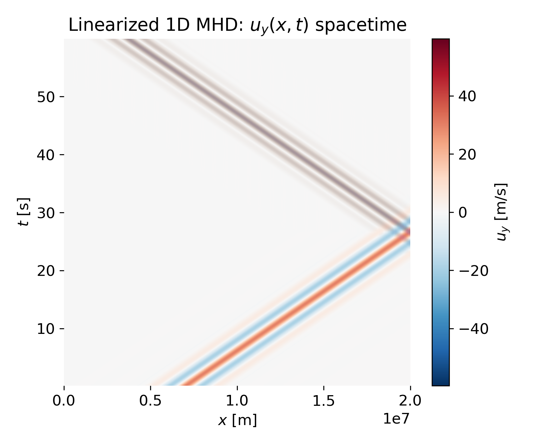
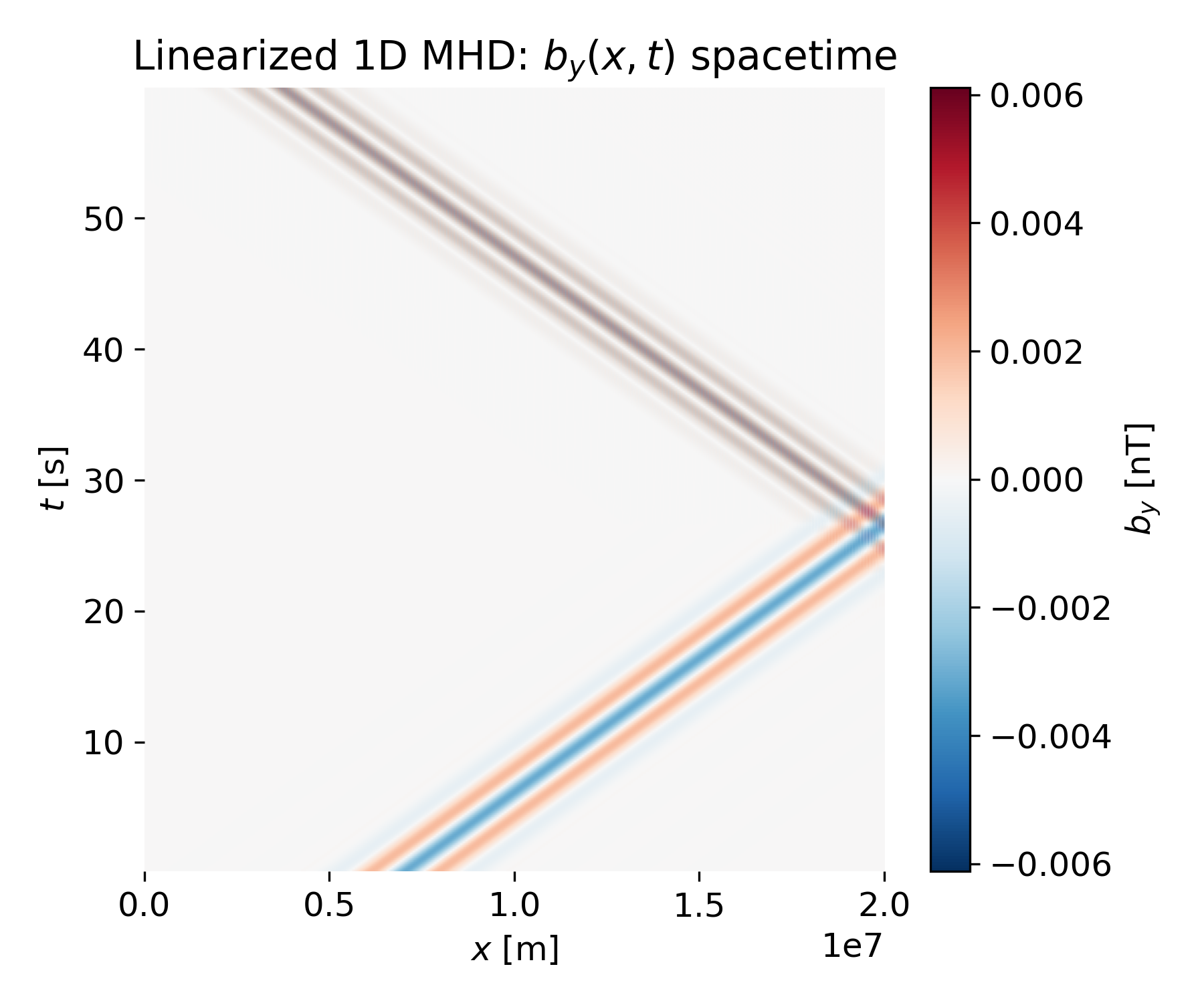
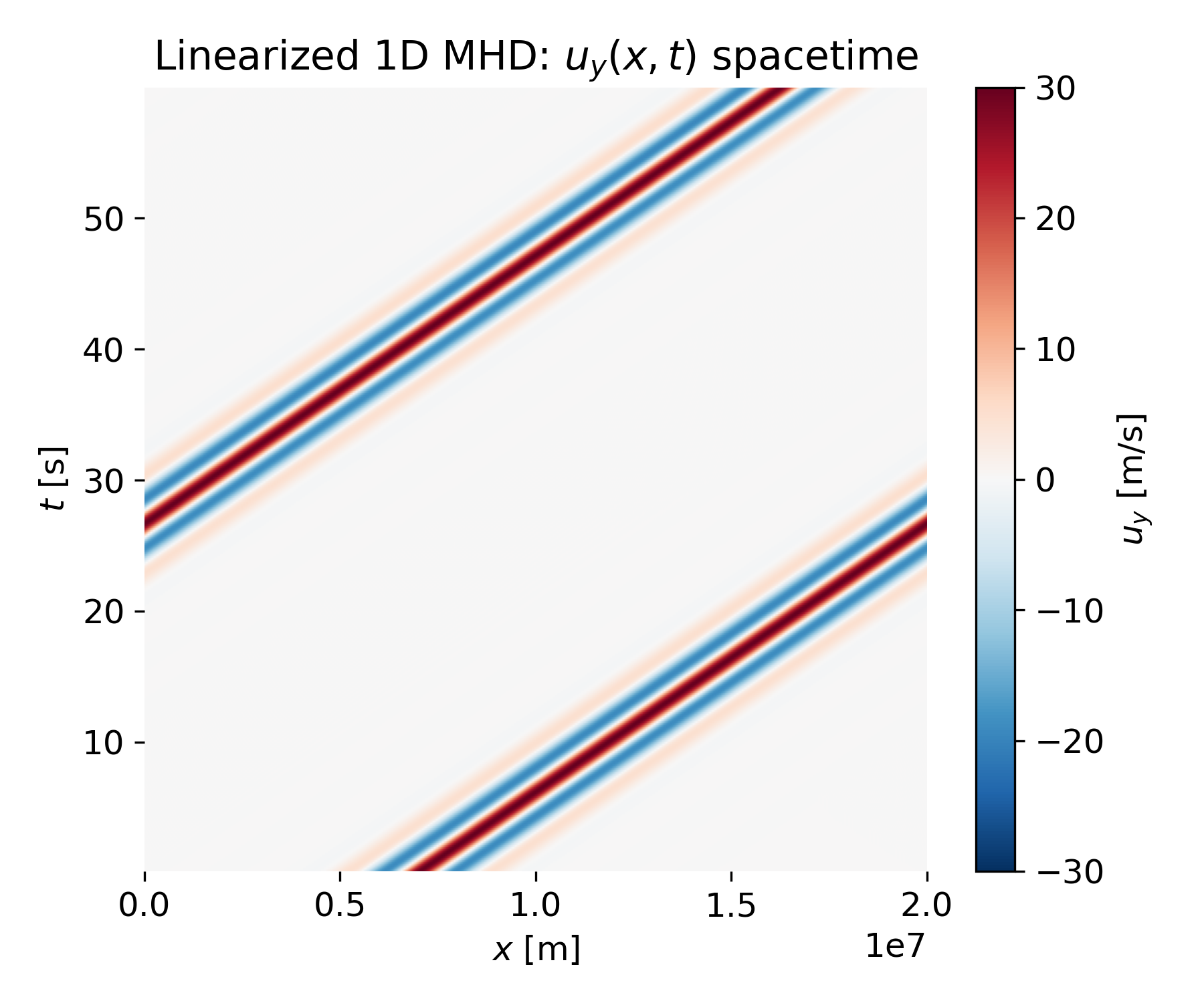
Left: Linearized 1D MHD: $u_y(x,t)$ spacetime for reflecting boundary conditions. The color-coded spacetime plot shows a localized Alfvén wave packet propagating diagonally across the domain. The slope of the diagonal features corresponds to the Alfvén speed $v_A$, confirming nondispersive propagation as expected from linearized MHD. When the packet reaches the right boundary, it is reflected, producing a second diagonal branch with opposite slope. – Right: Linearized 1D MHD: $b_y(x,t)$ spacetime for reflecting boundary conditions. The magnetic perturbation exhibits the same spacetime structure as the velocity field, with identical propagation speed and reflection behavior. This close correspondence reflects the Alfvénic coupling between $u_y$ and $b_y$, where both fields propagate together at $v_A$.

These spacetime plots already show the essential physics: A single Alfvén wave packet traveling at constant speed, reflecting at the boundary, and generating a counterpropagating wave. The reflection leads to overlap between incoming and reflected packets, which is explored in more detail in snapshot plots.

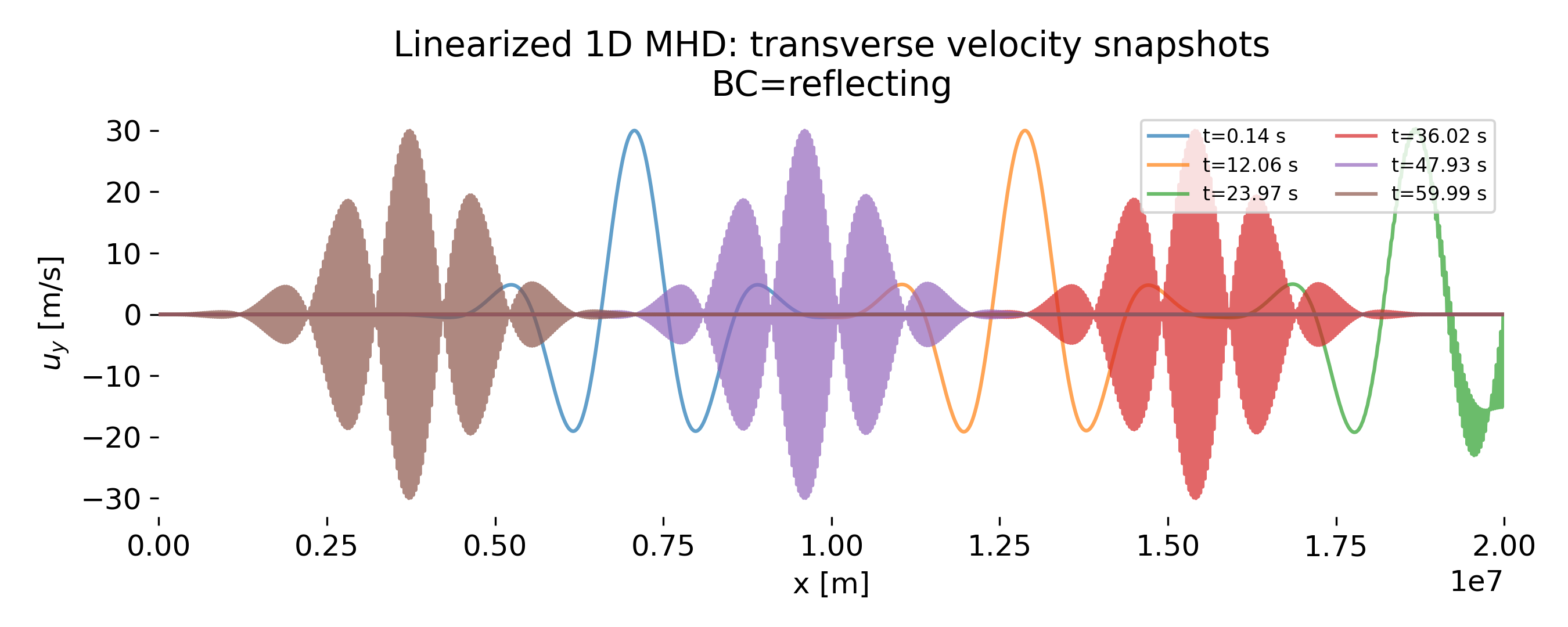
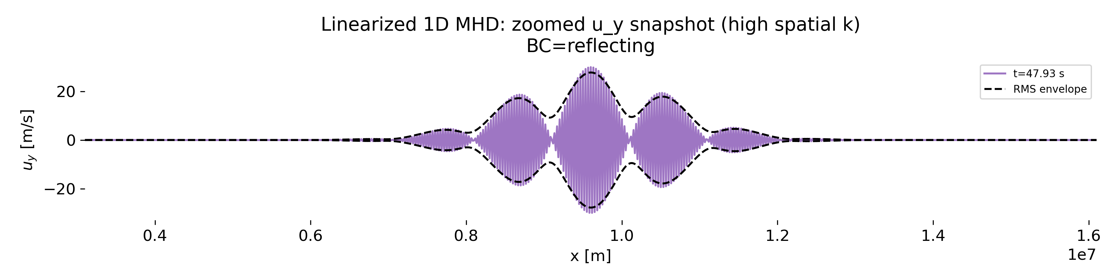
Top: Transverse velocity snapshots $u_y(x)$ at selected times for reflecting boundary conditions. Each curve corresponds to a different time and shows the instantaneous spatial structure of the wave packet. While the overall envelope remains localized, some snapshots display very rapid spatial oscillations within the packet. – Bottom: Zoomed $u_y(x)$ snapshot highlighting high spatial wavenumber content. The elongated spatial window resolves the fast carrier oscillations. The dashed curves indicate a local RMS envelope, plotted only as a visual guide to the packet extent. The envelope does not coincide exactly with the instantaneous extrema of $u_y$, which is expected: It represents a local energy measure, whereas the oscillatory signal carries phase information. Importantly, the envelope remains smooth and localized, confirming that the packet itself has not fragmented.

The zoomed snapshot plot reveals high-frequency oscillations within the overlapping region of incoming and reflected waves. At first glance, these high-frequency oscillations might suggest the emergence of shorter-wavelength waves. However, they are a direct consequence of linear superposition. After reflection, left- and right-propagating Alfvén waves coexist. Their interference produces a standing-wave–like pattern with an apparently shorter spatial scale, even though each constituent wave still satisfies the same Alfvén dispersion relation.

Let’s have a closer look at the magnetic field snapshots:

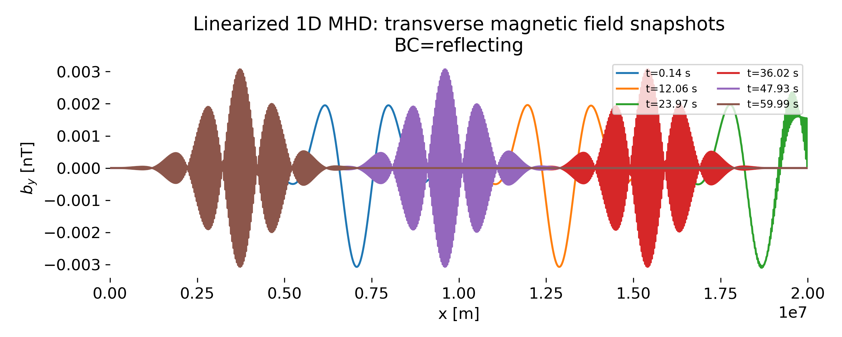
Transverse magnetic field snapshots $b_y(x)$ at selected times. The magnetic perturbation shows the same qualitative behavior as the velocity field: localized packets, reflection at the boundary, and interference-induced high-frequency oscillations in overlapping regions.

A direct comparison between the $u_y$ and $b_y$ snapshots reinforces the Alfvénic nature of the waves. The spatial locations of peaks and nodes coincide, and the packets propagate with the same apparent speed inferred from the spacetime plots. The relative amplitudes of $u_y$ and $b_y$ are consistent with Alfvén wave scaling, $|b_y| \sim \sqrt{\mu_0 \rho_0}\,|u_y|$, up to the chosen normalization. This confirms that the simulation preserves the correct phase relation and propagation speed between velocity and magnetic field fluctuations.

Taken together, the reflecting-boundary case demonstrates clean Alfvén propagation, reflection-induced generation of counterpropagating waves, and linear interference patterns that can temporarily mimic shorter wavelengths without invoking additional physics.

Periodic boundary conditions

For periodic boundaries, we restrict attention to a single spacetime plot:

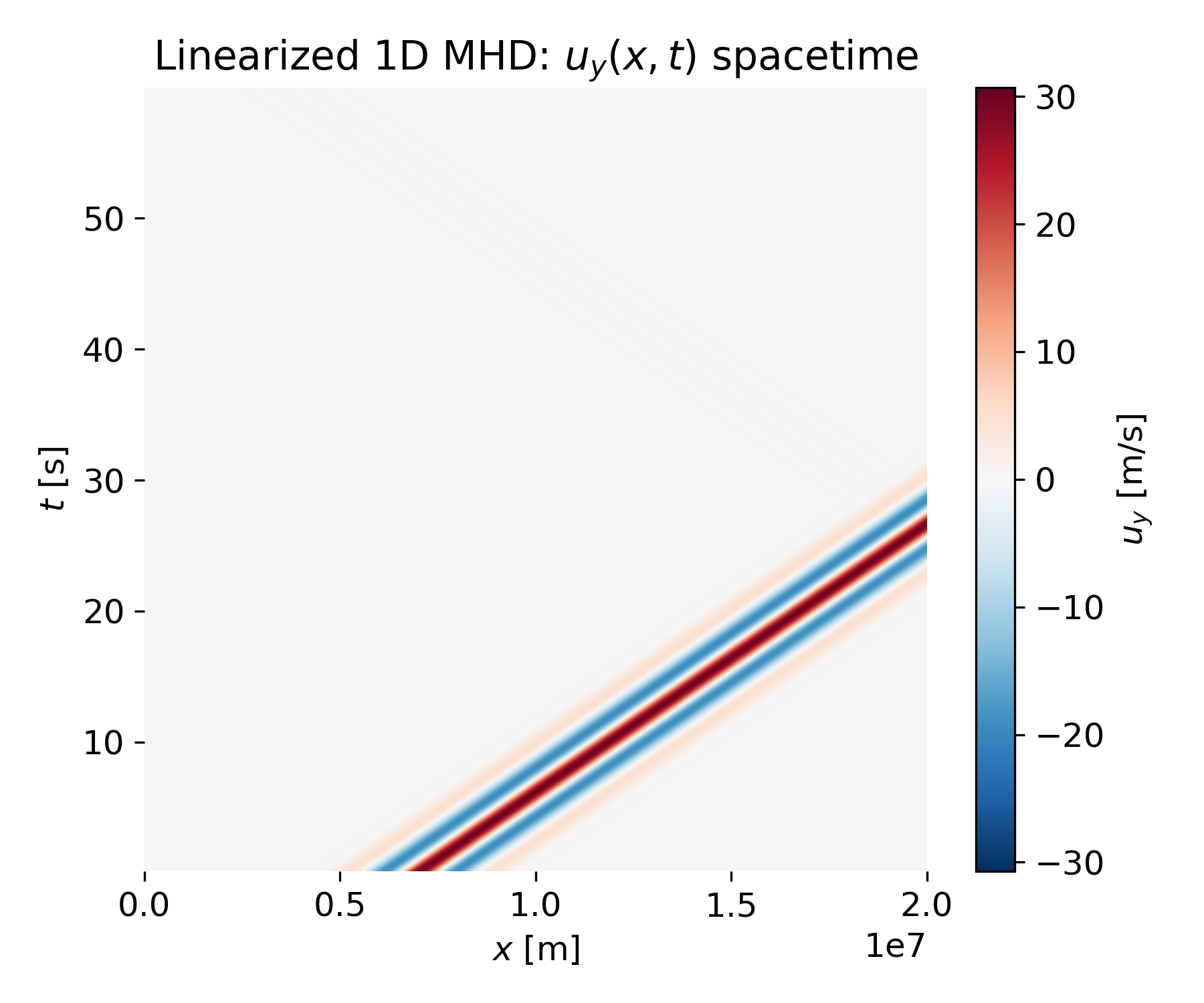
Linearized 1D MHD: $u_y(x,t)$ spacetime. Here, the wave packet exits the domain on one side and immediately re-enters on the opposite side. The spacetime diagram therefore shows uninterrupted diagonal bands wrapping around the domain.

Compared to the reflecting case, no reflected branch appears and no overlap between counterpropagating waves occurs. The result is a single family of parallel diagonal traces, corresponding to pure translation at constant speed $v_A$. Snapshot plots in this case show a single traveling packet at all times, without the high-frequency interference patterns seen for reflecting boundaries.

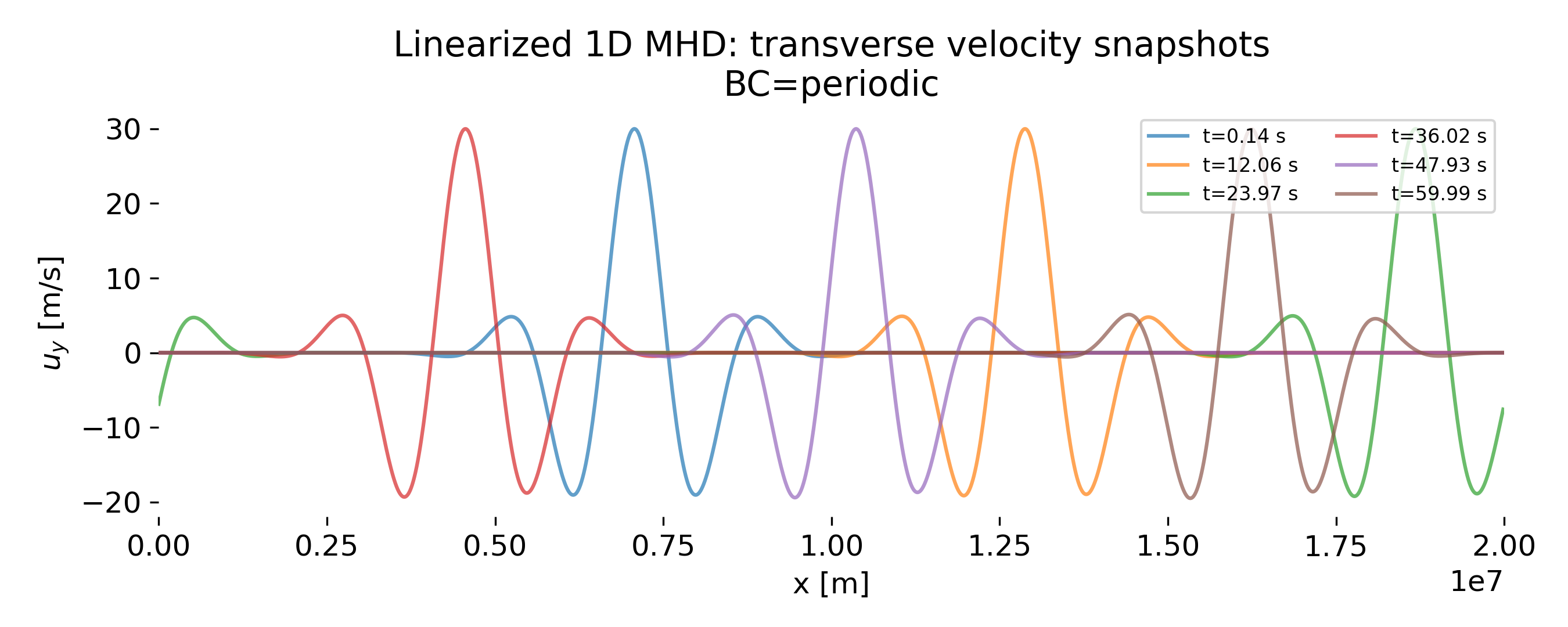Transverse velocity snapshots $u_y(x)$ at selected times for periodic boundary conditions. Each snapshot shows the wave packet moving through the domain without distortion or interference, consistent with pure Alfvénic propagation under periodic boundaries.

Open boundary conditions

Finally, we consider open (radiation-like) boundaries, again focusing on a single spacetime plot:

Linearized 1D MHD: $u_y(x,t)$ spacetime. The wave packet propagates toward the boundary and then leaves the computational domain with minimal reflection. In the spacetime plot, the diagonal trace simply terminates at the boundary, and no counterpropagating branch appears.

This behavior contrasts sharply with the reflecting case and demonstrates that the open boundary condition effectively suppresses artificial reflections. After the packet exits, the interior of the domain remains essentially undisturbed.

Summary of numerical results

Across all boundary conditions, the spacetime plots confirm nondispersive Alfvén propagation at the Alfvén speed with tightly coupled velocity and magnetic field perturbations. Reflecting boundaries introduce interference and standing-wave–like patterns through linear superposition, periodic boundaries enforce continuous translation, and open boundaries allow clean wave escape. The apparent complexity of some snapshot plots is therefore a boundary-induced effect rather than a change in the underlying wave physics.

Summary

The Alfvén wave is the canonical wave mode of magnetized plasmas. Its mathematical description in linearized magnetohydrodynamics is simple, transparent, and physically intuitive. At the same time, it provides a gateway to more sophisticated plasma physics, where dispersive corrections, kinetic effects, and wave particle interactions enrich the picture.

In the next step, this analytical foundation can be complemented by explicit numerical simulations of one dimensional Alfvén wave propagation, making the connection between equations, physical intuition, and observable wave dynamics explicit.

Update and code availability: This post and its accompanying Python code were originally drafted in 2020 and archived during the migration of this website to Jekyll and Markdown. In January 2026, I substantially revised and extended the code. The updated and cleaned-up implementation is now available in this new GitHub repositoryꜛ. Please feel free to experiment with it and to share any feedback or suggestions for further improvements.

References and further reading

• Wolfgang Baumjohann and Rudolf A. Treumann, Basic Space Plasma Physics, 1997, Imperial College Press, ISBN: 1-86094-079-X
• Treumann, R. A., Baumjohann, W., Advanced Space Plasma Physics, 1997, Imperial College Press, ISBN: 978-1-86094-026-2
• Stix, T. H., Waves in Plasmas, 1997, American Institute of Physics, ISBN: 978-0883188590
• Hannes Alfvén, Cosmical Electrodynamics, 1963, Nelson Thornes Ltd, ISBN: 978-0198512011
• Thomas J. M. Boyd & J. J. Sanderson, The Physics of Plasmas, 2003, Cambridge University Press, ISBN: 978-0521459129
• Paul A. Sturrock, Plasma Physics: An Introduction to the Theory of Astrophysical, Geophysical and Laboratory Plasmas, 2008, Cambridge University Press, ISBN: 978-0521448109
• Eric Priest, Solar Magnetohydrodynamics, 1982, Springer, ISBN: 978-9027713742
• Donald A. Gurnett & Amitava Bhattacharjee, Introduction to Plasma Physics with Space and Laboratory Applications, 2014, Cambridge University Press, ISBN: 978-7301245491
• Joachim Saur, Sascha Janser, Anne Schreiner, George Clark, Barry H. Mauk, Peter Kollmann, Robert W. Ebert, Frederic Allegrini, Jamey R. Szalay, Stavros Kotsiaros, Wave-particle interaction of Alfvén waves in Jupiter’s magnetosphere: Auroral and magnetospheric particle acceleration, 2018, Journal of Geophysical Research: Space Physics, 123, 9560–9573. DOI: 10.1029/2018JA025948ꜛ
• Chané, E., J. Saur, F. M. Neubauer, J. Raeder, and S. Poedts, Observational evidence of Alfvén wings at the Earth, 2012, J. Geophys. Res., 117, A09217, DOI: 10.1029/2012JA017628
• Hinton, P. C., Bagenal, F., & Bonfond, B., Alfvén wave propagation in the Io plasma torus, 2019, Geophysical Research Letters, 46, 1242–1249. DOI: 10.1029/2018GL081472ꜛ