Plasma waves in space plasmas

Space plasmas support a rich spectrum of collective wave phenomena that have no direct analogue in neutral fluids. These waves arise from the self consistent coupling between charged particles and electromagnetic fields and therefore occupy a conceptual boundary between fluid descriptions and fully kinetic theory. On sufficiently large spatial and temporal scales, plasma waves can often be understood as perturbations of a conducting fluid governed by magnetohydrodynamics. On smaller scales, or whenever resonant interactions between particles and fields become important, a kinetic description in terms of distribution functions and phase space dynamics is unavoidable. Plasma waves thus provide a natural bridge between macroscopic magnetofluid behavior and microscopic particle physics.

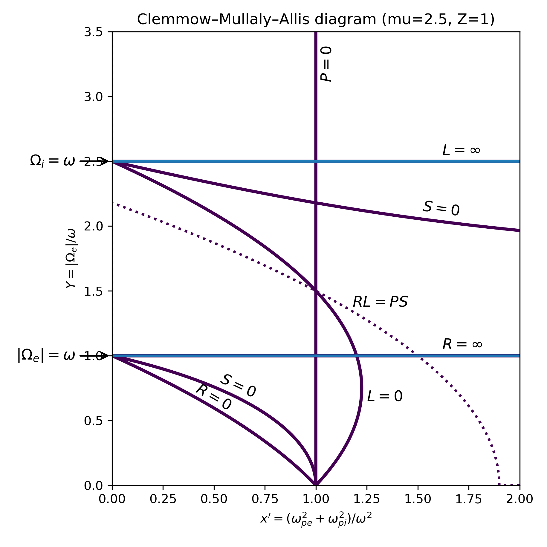
Clemmow–Mullaly–Allis (CMA) diagram for a cold, two-component plasma. Plasma waves arise from the self consistent coupling between charged particles and electromagnetic fields. The CMA diagram provides a global overview of propagation regimes, cutoffs, and resonances that underlie all cold plasma wave modes. Shown are the boundary curves of the cold plasma dispersion relation in the dimensionless parameter space $x’ = (\omega_{pe}^2 + \omega_{pi}^2)/\omega^2$ and $Y = |\Omega_e|/\omega$. The diagram is constructed from the Stix parameters $P$, $R$, $L$, and $S$ and their combinations. Solid curves indicate the conditions $P=0$, $R=0$, $L=0$, and $S=0$, while the dotted curve corresponds to $RL = PS$. Horizontal lines mark the electron and ion cyclotron resonances $|\Omega_e|=\omega$ and $\Omega_i=\omega$. These boundaries partition parameter space into distinct propagation regimes with different numbers and types of electromagnetic wave solutions. The CMA diagram provides a global, qualitative classification of cold plasma wave behavior independent of any specific $\omega(k)$ dispersion curve. The figure is adapted from Stix (1997), Waves in Plasmas, American Institute of Physics. We will discuss it in more detail throughout this post. The Python code used to generate the diagram is available on GitHubꜛ.

In space environments such as the solar wind, planetary magnetospheres, and astrophysical jets, plasma waves play a central role in energy transport, particle acceleration, heating, and the onset of instabilities. Observed fluctuations in magnetic and electric fields are very often wave like in character and encode information about plasma parameters, background magnetic fields, and non equilibrium particle populations. A systematic understanding of plasma waves is therefore essential for interpreting in situ spacecraft measurements and for connecting observations to theoretical models.

Waves at the interface of fluid and kinetic theory

The most general description of a collisionless plasma is given by the Vlasov Maxwell system. For each species $s$ with charge $q_s$ and mass $m_s$, the distribution function $f_s(\mathbf{x},\mathbf{v},t)$ evolves according to

\[\partial_t f_s + \mathbf{v}\cdot\nabla f_s + \frac{q_s}{m_s}(\mathbf{E} + \mathbf{v}\times\mathbf{B})\cdot\nabla_{\mathbf{v}} f_s = 0,\]

coupled to Maxwell’s equations for $\mathbf{E}$ and $\mathbf{B}$. Linearizing around a homogeneous equilibrium $f_{s0}(\mathbf{v})$ and assuming plane wave perturbations $\propto \exp[i(\mathbf{k}\cdot\mathbf{x}-\omega t)]$ leads to a homogeneous system of equations for the field amplitudes. Non trivial solutions exist only if

\[\det!\left| \mathbf{D}(\omega,\mathbf{k}) \right| = 0,\]

where $\mathbf{D}$ is the dielectric tensor. This dispersion relation contains all linear plasma waves and their damping or growth rates.

Fluid theory emerges by taking velocity moments of the Vlasov equation. Truncating the moment hierarchy and closing it by assumptions on pressure or temperature leads to magnetohydrodynamics. Linearized MHD describes perturbations of density $\rho$, velocity $\mathbf{u}$, magnetic field $\mathbf{B}$, and pressure $p$ around a stationary equilibrium. Plasma waves therefore occupy the overlap region where the assumptions behind such closures can be tested against kinetic reality.

Linear theory and the cold plasma approximation

In the cold plasma approximation, thermal velocities are neglected and each species responds coherently to electromagnetic perturbations. The linearized equation of motion for species $s$ is

\[- i \omega \mathbf{v}_s = \frac{q_s}{m_s}(\mathbf{E} + \mathbf{v}_s \times \mathbf{B}_0),\]

which can be solved algebraically for $\mathbf{v}_s$ in terms of $\mathbf{E}$. Inserting the resulting current into Maxwell’s equations yields a wave equation of the form

\[\left[ k^2 c^2 \mathbf{I} - \mathbf{k}\mathbf{k}c^2 - \omega^2 \boldsymbol{\varepsilon}(\omega) \right]\cdot\mathbf{E} = 0,\]

where $\boldsymbol{\varepsilon}$ is the cold plasma dielectric tensor. The condition for non trivial solutions leads to the Appleton Hartree dispersion relation for electromagnetic waves in a magnetized plasma.

Despite its simplicity, the cold plasma model already predicts multiple wave branches, polarization states, and resonance frequencies. These features provide a baseline classification scheme widely used in space plasma diagnostics.

Fundamental wave modes in magnetized plasmas

Electromagnetic ion cyclotron waves appear near the ion gyrofrequency $\Omega_i = q_i B_0/m_i$. In the cold plasma limit and for parallel propagation, their dispersion relation is approximately

\[\omega \approx \Omega_i + \frac{k^2 v_A^2}{\Omega_i},\]

where $v_A$ is the Alfvén speed. These waves are circularly polarized and strongly tied to ion dynamics.

Alfvén waves arise as transverse solutions of the linearized ideal MHD equations. Combining Faraday’s law with the momentum equation yields the Alfvén wave equation

\[\partial_t^2 \mathbf{u}_\perp = v_A^2 \partial_\parallel^2 \mathbf{u}_\perp,\]

with the dispersion relation

\[\omega = k_\parallel v_A.\]

They are incompressible, nondispersive, and propagate strictly along magnetic field lines in ideal MHD.

Magnetosonic waves result from the coupling between compressibility and magnetic pressure. Linearizing the MHD equations yields the dispersion relation

\[\omega^2 = \frac{1}{2}k^2\left(v_A^2 + c_s^2\right) \pm \frac{1}{2}k^2\sqrt{(v_A^2 + c_s^2)^2 - 4v_A^2 c_s^2 \cos^2\theta},\]

corresponding to fast and slow branches, where $c_s$ is the sound speed and $\theta$ the angle between $\mathbf{k}$ and $\mathbf{B}_0$.

Whistler waves occupy the high frequency electromagnetic branch dominated by electron inertia. For parallel propagation in a cold plasma, their dispersion relation reduces to

\[\omega = \frac{\Omega_e k^2 c^2}{\omega_{pe}^2},\]

illustrating their strong dispersion and sensitivity to electron dynamics.

Warm plasma effects and kinetic corrections

Finite temperature modifies plasma waves through pressure forces, finite Larmor radius effects, and resonant interactions. In kinetic theory, these corrections enter through velocity space integrals of the form

\[\int \frac{\mathbf{k}\cdot\nabla_{\mathbf{v}} f_{s0}}{\omega - \mathbf{k}\cdot\mathbf{v} - n\Omega_s} , d^3v,\]

which generate Landau and cyclotron resonances. These resonances lead to damping or growth even in collisionless plasmas and fundamentally alter wave propagation.

Warm plasma theory predicts additional wave branches and smooth transitions between fluid modes and kinetic modes. Alfvén waves, for instance, continuously evolve into kinetic Alfvén waves when perpendicular wavelengths approach the ion gyroradius, introducing parallel electric fields absent in ideal MHD.

Dispersion relations and $\omega(k)$ diagrams

Dispersion relations encode the complete linear wave physics of a plasma. Plotting $\omega(k)$ makes phase velocities $v_\phi = \omega/k$, group velocities $v_g = \partial\omega/\partial k$, cutoff regions, and mode coupling directly visible. In space plasma physics, measured field spectra are routinely compared to theoretical dispersion curves to infer plasma parameters such as density, temperature, composition, and background magnetic field strength.

Such $\omega(k)$ diagrams also provide a clear visualization of where fluid descriptions remain valid and where kinetic effects become unavoidable. They therefore form a natural bridge between magnetohydrodynamic intuition and the full electromagnetic response of a collisionless plasma.

The Clemmow–Mullaly–Allis diagram

Before turning to explicit $\omega(k)$ dispersion curves, it is useful to introduce a complementary representation of cold plasma wave physics: The Clemmow–Mullaly–Allis (CMA) diagram. Rather than plotting frequency versus wavenumber, the CMA diagram maps the structure of the cold plasma dispersion relation in a reduced, dimensionless parameter space. It provides a global overview of propagation regimes, cutoffs, and resonances that underlie all cold plasma wave modes. The figure at the top of this post shows an example of a CMA diagram for a two component plasma.

Historically, the CMA diagram was developed as a classification tool for electromagnetic waves in magnetized plasmas and is discussed extensively in standard references such as Stix. Its strength lies in making the topology of the dispersion relation visible independently of any particular wave vector or frequency scale.

Let’s briefly summarize its construction and interpretation. The CMA diagram is constructed from the cold plasma dielectric tensor written in terms of the Stix parameters $R$, $L$, $S$, $D$, and $P$. For a collisionless, homogeneous plasma with background magnetic field $\mathbf{B}_0$, these parameters are defined as

\[\begin{aligned} R &= 1 - \sum_s \frac{\omega_{ps}^2}{\omega(\omega + \Omega_s)},\\ L &= 1 - \sum_s \frac{\omega_{ps}^2}{\omega(\omega - \Omega_s)},\\ P &= 1 - \sum_s \frac{\omega_{ps}^2}{\omega^2}, \end{aligned}\]

and

\[\begin{aligned} S &= \frac{1}{2}(R + L), \\ D &= \frac{1}{2}(R - L). \end{aligned}\]

Here $\omega_{ps}$ and $\Omega_s$ are the plasma and cyclotron frequencies of species $s$. The quantities $R$ and $L$ correspond to right-hand and left-hand circularly polarized responses for parallel propagation, while $P$ describes the purely longitudinal (electrostatic) response.

In the CMA construction, the dispersion relation is not solved explicitly for $\omega(k)$. Instead, the conditions under which propagating solutions exist are analyzed algebraically. Key boundaries in parameter space arise when one of the Stix parameters vanishes or diverges, or when combinations of them become equal. Of particular importance are the conditions

\[P = 0, \qquad R = 0, \qquad L = 0, \qquad S = 0,\]

as well as the mixed condition

\[RL = PS.\]

These relations define curves in a two-dimensional, dimensionless parameter space.

A common choice of CMA coordinates is

\[\begin{aligned} x' &= \frac{\omega_{pe}^2 + \omega_{pi}^2}{\omega^2}, \\ Y &= \frac{|\Omega_e|}{\omega}, \end{aligned}\]

where $x’$ measures the total plasma inertia relative to the wave frequency, and $Y$ measures the strength of magnetization. Resonances appear as horizontal lines at $|\Omega_e|=\omega$ and $\Omega_i=\omega$, while electrostatic cutoffs appear as vertical lines at $P=0$.

Interpretation of the diagram

When the boundary curves are plotted in the $(x’,Y)$ plane, they divide the diagram into a finite number of distinct regions, typically sixteen for a two-component plasma. Each region corresponds to a different qualitative structure of the cold plasma dispersion relation. Crossing a boundary changes the number of propagating modes, their polarization, or their accessibility.

The line $P=0$ marks the plasma frequency cutoff, separating regions where purely longitudinal oscillations are allowed from those where they are forbidden. The conditions $R=0$ and $L=0$ correspond to resonances of right-hand and left-hand polarized electromagnetic waves. The line $S=0$ separates regimes dominated by transverse electromagnetic response from those where longitudinal and transverse components are strongly coupled.

The curve defined by $RL=PS$ plays a central role in the topology of the dispersion relation. It marks transitions where wave branches reconnect or change character, and it is responsible for the characteristic bending and folding of dispersion surfaces in wave-normal space.

Importantly, the CMA diagram does not describe individual wave modes in isolation. Instead, it encodes the full structure of the cold plasma dispersion relation and its allowed solutions. Familiar waves such as Alfvén waves, ion cyclotron waves, magnetosonic modes, and whistler waves correspond to particular paths through this parameter space as $\omega$ and $k$ are varied.

Conceptual role of the CMA diagram

The CMA diagram provides a qualitative map of cold plasma wave physics that complements explicit $\omega(k)$ plots. While $\omega(k)$ diagrams show how specific modes propagate for given plasma parameters, the CMA diagram explains why those modes exist in the first place, where they terminate, and how different branches are connected.

In this sense, the CMA diagram serves as a unifying framework for understanding the topology of cold plasma dispersion relations. It makes clear that the complexity seen in $\omega(k)$ diagrams is not accidental, but a direct consequence of the algebraic structure of the dielectric tensor. In the following section, this abstract classification is made concrete by computing explicit $\omega(k)$ dispersion relations using the Appleton–Hartree formalism for specific plasma environments.

Cold plasma electromagnetic dispersion via the Appleton–Hartree formalism

As a general framework for constructing $\omega(k)$ diagrams, the Appleton–Hartree formalism describes the full electromagnetic dispersion relation of a cold, magnetized plasma for arbitrary propagation angle. Rather than focusing on individual wave modes, this approach yields the complete linear spectrum in a unified, angle dependent representation. Familiar plasma waves such as Alfvén waves, ion cyclotron waves, magnetosonic modes, and whistler waves then appear as different asymptotic limits of the same underlying electromagnetic theory.

The formalism presented in this section is fully general and independent of any specific plasma environment. Only the choice of plasma parameters such as density, magnetic field strength, and species composition determines which parts of the spectrum are realized in a given physical setting.

Let’s briefly summarize the derivation. In a homogeneous, collisionless cold plasma with a background magnetic field $\mathbf{B}_0$, linearization of the fluid equations for each species and coupling to Maxwell’s equations leads to the wave equation

\[\left[k^2 c^2 \mathbf{I} - \mathbf{k}\mathbf{k} c^2 - \omega^2 \boldsymbol{\varepsilon}(\omega)\right]\cdot\mathbf{E} = 0,\]

where $\boldsymbol{\varepsilon}(\omega)$ is the cold plasma dielectric tensor. Nontrivial solutions require the determinant of the operator in brackets to vanish. For oblique propagation at an angle $\theta$ between the wave vector $\mathbf{k}$ and $\mathbf{B}_0$, this condition reduces to a quadratic equation for the refractive index squared $n^2 = c^2 k^2 / \omega^2$,

\[A n^4 - B n^2 + C = 0.\]

The coefficients are expressed in terms of the Stix parameters $R$, $L$, $S$, and $P$,

\[\begin{aligned} A &= S\sin^2(\theta) + P\cos^2(\theta), \\ B &= R L \sin^2(\theta) + P S (1 + \cos^2(\theta)), \\ C &= P R L, \end{aligned}\]

with

\[\begin{aligned} R &= 1 - \sum_s \frac{\omega_{ps}^2}{\omega(\omega + \Omega_s)},\\ L &= 1 - \sum_s \frac{\omega_{ps}^2}{\omega(\omega - \Omega_s)}, \\ P &= 1 - \sum_s \frac{\omega_{ps}^2}{\omega^2}. \end{aligned}\]

Here $\omega_{ps}$ and $\Omega_s$ denote the plasma and cyclotron frequencies of species $s$. Solving the quadratic yields two electromagnetic branches,

\[n^2_{\pm}(\omega) = \frac{B \pm \sqrt{B^2 - 4AC}}{2A}.\]

Rather than solving implicitly for $\omega(k)$, $\omega(k)$ diagrams are constructed parametrically. The frequency $\omega$ is sampled over a broad range spanning ion to electron scales. For each $\omega$ and fixed propagation angle $\theta$, the corresponding $n^2(\omega)$ is evaluated and the wavenumber obtained from

\[k(\omega) = \frac{\omega}{c}\sqrt{n^2(\omega)}.\]

Only intervals where $n^2$ is real and positive correspond to propagating electromagnetic waves and appear in the diagram. Regions where $n^2$ becomes negative or complex correspond to evanescent solutions, cutoffs, or resonance boundaries intrinsic to the cold plasma response.

I’ve written a Python implementation of this procedure that computes and plots the full cold plasma electromagnetic dispersion relation for arbitrary parameter choices. You can find the code in this GitHub repository.

Appleton–Hartree dispersion for solar wind–like parameters

As a first concrete example, the Appleton–Hartree formalism is applied to a parameter set representative of the solar wind and magnetosheath. This regime provides a physically transparent baseline in which thermal effects are often subdominant for large scale fluctuations, and the cold plasma approximation already captures the essential structure seen in spacecraft observations.

The parameters used are

Parameter	Symbol	Value	Unit
Magnetic field strength	$B_0$	$50$	nT
Speed of light	$c$	$299\,792\,458$	m/s
Vacuum permittivity	$\varepsilon_0$	$8.854 \times 10^{-12}$	F/m
Vacuum permeability	$\mu_0$	$4\pi \times 10^{-7}$	H/m
Elementary charge	$e$	$1.602 \times 10^{-19}$	C
Electron mass	$m_e$	$9.109 \times 10^{-31}$	kg
Proton mass	$m_p$	$1.673 \times 10^{-27}$	kg
Number density	$n_e$	$5.0$	cm$^{-3}$
Electron charge	$q_e$	$-e$	C
Proton charge	$q_p$	$+e$	C

The resulting $\omega(k)$ diagram is shown below:

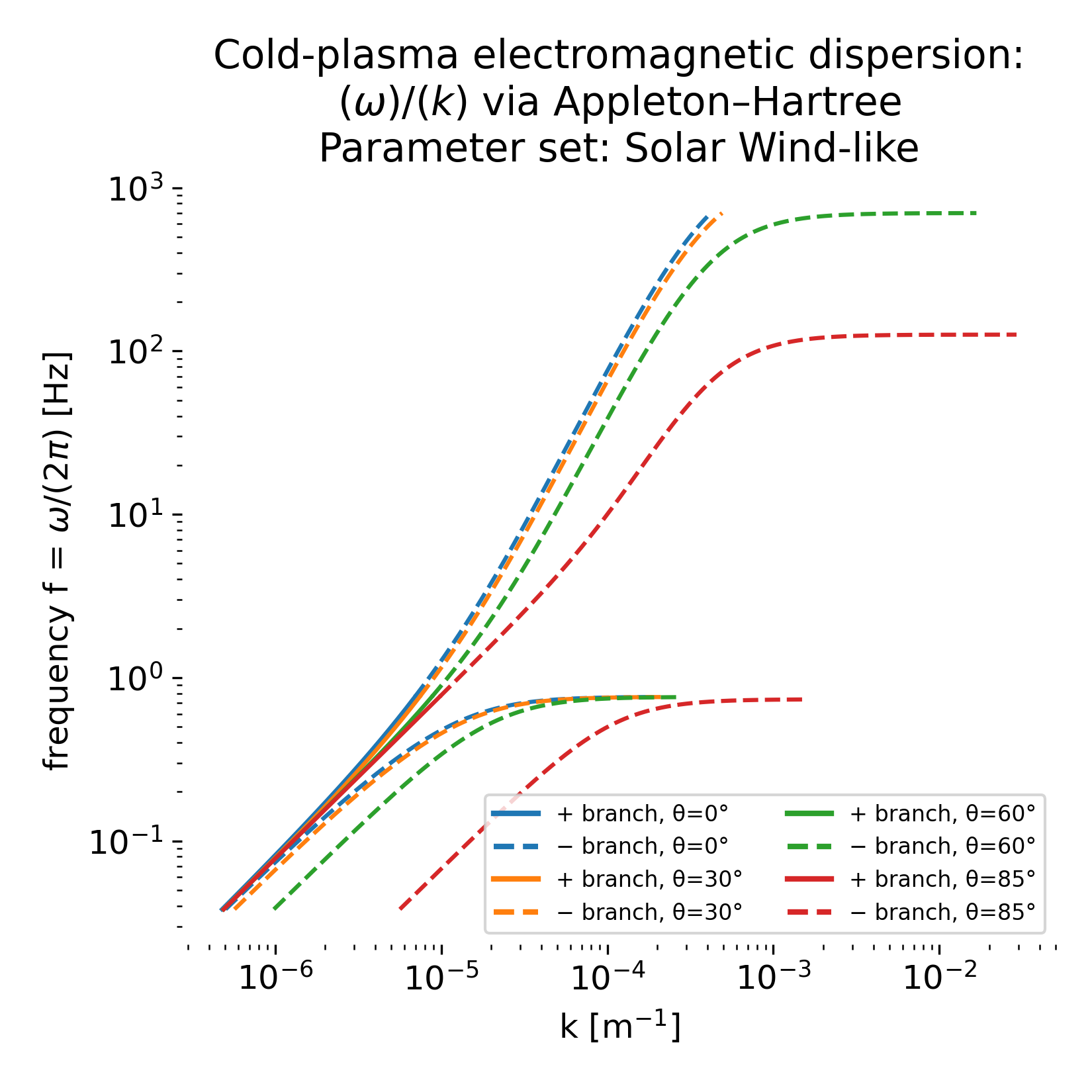
Cold plasma electromagnetic dispersion relation $\omega(k)$ computed from the Appleton–Hartree formalism for solar wind–like parameters. Shown are the two electromagnetic branches $n^2_\pm$ for oblique propagation at four angles $\theta$ between the wave vector $\mathbf{k}$ and the background magnetic field $\mathbf{B}_0$. For each angle, the plus branch is plotted as a solid line and the minus branch as a dashed line, using the same color to emphasize their common angular origin. At small wavenumbers, all curves approach the Alfvénic limit with approximately linear $\omega \propto k_\parallel$ scaling. At higher frequencies, dispersive behavior and branch separation become prominent, reflecting cyclotron resonances and cutoff regions intrinsic to the cold plasma dielectric response. Apparent gaps and terminations correspond to frequency intervals where $n^2$ becomes negative or complex and propagating electromagnetic solutions no longer exist. The full, reproducible Python code used to generate this figure is available in the accompanying GitHub repository.

The resulting $\omega(k)$ diagram represents the complete cold plasma electromagnetic spectrum rather than individual wave modes plotted in isolation. Several characteristic features are evident.

At low frequencies and small wavenumbers, all branches approach an approximately linear relation $\omega \propto k_\parallel$. This is the Alfvénic limit, where the full electromagnetic description smoothly reduces to the familiar magnetohydrodynamic Alfvén wave. The weak dependence on propagation angle in this regime reflects the dominance of field aligned dynamics and the validity of a fluid description.

At intermediate frequencies, the dispersion curves bend and separate as electromagnetic effects become important. The splitting between the two branches and their increasing angular dependence arise from the anisotropic dielectric response encoded in the Stix parameters. In this regime, magnetosonic like behavior and the low frequency limit of the whistler branch coexist within the same formalism.

In contrast to schematic textbook plots, the present $\omega(k)$ representation does not show perfectly horizontal lines at the ion cyclotron frequency. Instead, the curves exhibit abrupt terminations and apparent jumps. These features reflect the fact that the dispersion relation is constructed parametrically in $\omega$. Near cyclotron resonances, terms of the form $(\omega - \Omega_i)^{-1}$ enter the dielectric tensor, causing $n^2$ to diverge or change sign. As a result, the mapping $k(\omega)$ ceases to be single valued and real propagating solutions no longer exist beyond these points. The apparent discontinuities therefore mark resonance boundaries and cutoff regions rather than numerical artifacts.

At higher frequencies, the right hand polarized electromagnetic branch separates clearly and shows strong dispersion. Its low frequency part corresponds to the whistler wave, while at larger $\omega$ it transitions toward electron scale dynamics. The pronounced dependence on $\theta$ reflects increasing coupling between transverse and longitudinal field components for oblique propagation.

The gaps in the diagram are regions where $n^2$ becomes negative or complex. In these intervals, the cold plasma does not support propagating electromagnetic waves and the solutions are evanescent. Their presence highlights the intrinsic cutoff structure of magnetized plasmas even in the absence of kinetic effects.

Summary:
This representation makes explicit that Alfvén waves, ion cyclotron effects, magnetosonic like behavior, and whistler waves are not independent phenomena but interconnected manifestations of a single electromagnetic dispersion relation. The diagram also illustrates why plasma waves occupy the boundary between fluid and kinetic descriptions. Magnetohydrodynamic modes emerge naturally as low frequency limits, while resonances, cutoffs, and branch terminations already signal where kinetic physics becomes essential.

For clarity, the numerical implementation used to generate this figure is not shown here. The full, reproducible Python code is provided in the accompanying GitHub repositoryꜛ, where parameter choices, angular dependence, and frequency ranges can be explored interactively.

Appleton–Hartree dispersion for magnetosheath–like parameters

As a second example, the same Appleton–Hartree construction is applied to plasma parameters representative of the terrestrial magnetosheath. Compared to the solar wind–like baseline, this regime is characterized by higher densities and a weaker background magnetic field, reflecting the compressed and heated plasma downstream of the bow shock.

The parameters used here are

Parameter	Symbol	Value	Unit
Magnetic field strength	$B_0$	$20$	nT
Number density	$n_e$	$30$	cm$^{-3}$
Electron charge	$q_e$	$-e$	C
Proton charge	$q_p$	$+e$	C
Electron mass	$m_e$	$9.109 \times 10^{-31}$	kg
Proton mass	$m_p$	$1.673 \times 10^{-27}$	kg

The according $\omega(k)$ diagram looks as follows:

Cold plasma electromagnetic dispersion relation $\omega(k)$ computed from the Appleton–Hartree formalism for magnetosheath-like parameters at Earth. Shown are the two electromagnetic branches $n^2_\pm$ for oblique propagation at four angles $\theta$ between the wave vector $\mathbf{k}$ and the background magnetic field $\mathbf{B}_0$. Solid lines denote the plus branch and dashed lines the minus branch, with matching colors indicating identical propagation angles. Compared to the solar wind–like case, characteristic frequencies and branch terminations are shifted to lower values due to the higher density and weaker magnetic field in the magnetosheath. The full, reproducible Python code used to generate this figure is available in the accompanying GitHub repositoryꜛ.

A quasi-neutral proton–electron plasma is assumed, and the dispersion relation is evaluated for the same set of propagation angles as in the solar wind–like case.

Qualitatively, the resulting $\omega(k)$ diagram closely resembles the solar wind–like spectrum, confirming that the overall topology of the cold plasma electromagnetic dispersion relation is robust across these near-Earth environments. At low frequencies and small wavenumbers, all branches again converge toward the Alfvénic limit, reflecting fluid-like behavior along the background magnetic field.

Quantitative differences arise from the altered parameter ratios. The increased density shifts characteristic frequencies downward, while the reduced magnetic field lowers the ion and electron cyclotron frequencies. As a result, branch separations, cutoffs, and terminations occur at smaller $\omega$ compared to the solar wind–like case. The stronger angular dependence seen at intermediate and higher frequencies reflects the enhanced role of anisotropy in the magnetosheath, where fluctuations are often more oblique and broadband.

As before, apparent gaps and abrupt terminations of the curves correspond to regions where $n^2$ becomes negative or complex. These mark cutoff regions and resonance boundaries intrinsic to the cold plasma dielectric response, not numerical artifacts. The magnetosheath thus provides a natural intermediate regime in which the same formalism connects smoothly to both the upstream solar wind and more extreme environments discussed below.

Appleton–Hartree dispersion for auroral acceleration region–like parameters (Earth)

The auroral acceleration region represents a qualitatively different cold-plasma regime than the solar wind and magnetosheath. The magnetic field is orders of magnitude stronger, while the density is much lower. As a result, the characteristic cyclotron frequencies are pushed upward and the dispersion diagram becomes dominated by pronounced resonance structure. In this environment, the cold-plasma approximation still provides a useful baseline for classifying electromagnetic branches, but it also makes very explicit where the idealized resonances of the model appear.

The parameters used here are

Parameter	Symbol	Value	Unit
Magnetic field strength	$B_0$	$50$	$\mu$T
Number density	$n_e$	$0.1$	cm$^{-3}$
Electron charge	$q_e$	$-e$	C
Proton charge	$q_p$	$+e$	C
Electron mass	$m_e$	$9.109 \times 10^{-31}$	kg
Proton mass	$m_p$	$1.673 \times 10^{-27}$	kg

The according $\omega(k)$ diagram looks as follows:

Cold plasma electromagnetic dispersion relation $\omega(k)$ computed from the Appleton–Hartree formalism for auroral acceleration region–like parameters at Earth. Shown are the two electromagnetic branches $n^2_\pm$ for oblique propagation at four angles $\theta$ between $\mathbf{k}$ and $\mathbf{B}_0$. Solid lines denote the plus branch and dashed lines the minus branch, with matching colors indicating identical propagation angles. Compared to solar wind and magnetosheath conditions, the much stronger magnetic field and lower density shift cyclotron and cutoff structure into the plotted range. The nearly horizontal plateaus correspond to cyclotron resonance regions where the cold plasma response becomes resonance dominated and the group velocity tends toward zero. The full, reproducible Python code used to generate this figure is available in the accompanying GitHub repositoryꜛ.

A quasi-neutral proton–electron plasma is assumed. Compared to the solar wind–like baseline, the most striking change in the $\omega(k)$ diagram is the appearance of extended, nearly horizontal segments. These plateaus are the cold-plasma signature of cyclotron resonance regions: the dielectric tensor contains terms with denominators $(\omega \pm \Omega_s)$, so that $n^2(\omega)$ becomes extremely large or changes sign near $\omega \simeq \Omega_s$. In the parametric representation $k(\omega) = (\omega/c)\sqrt{n^2(\omega)}$, this behavior translates into frequency intervals where $\omega$ varies only weakly while $k$ spans a broad range, which appears as a horizontal branch segment.

The diagram also shows that these plateau regions coexist with more fluid-like behavior at low $k$. At sufficiently small $\omega$ and $k$, the branches again approach an approximately linear scaling $\omega \propto k_\parallel$, consistent with the Alfvénic low-frequency limit. The key difference is that the auroral parameter ratios shift the resonance and cutoff structure into the frequency range plotted here, making the transition from fluid-like to strongly dispersive electromagnetic behavior far more abrupt than in the magnetosheath.

In physical terms, the horizontal plateaus and sharp branch terminations indicate frequency bands where propagating electromagnetic solutions are suppressed by cutoffs or replaced by resonance-dominated response. In a warm or kinetic theory these idealized features would be broadened by finite temperature and resonant wave–particle effects, but their location and qualitative role remain central for interpreting auroral wave spectra.

Appleton–Hartree dispersion for Io plasma torus–like parameters (Jupiter)

The Io plasma torus is a dense, multi-ion magnetospheric plasma in which heavy ions dominate the low-frequency electromagnetic response. Even within a cold-plasma description, the presence of multiple ion species introduces a qualitatively richer dispersion structure because each ion contributes its own cyclotron and plasma frequencies. The Appleton–Hartree framework is therefore particularly useful here as a compact way to visualize how composition reshapes the electromagnetic spectrum.

The parameters used here are

Parameter	Symbol	Value	Unit
Magnetic field strength	$B_0$	$2$	$\mu$T
Electron number density	$n_e$	$2000$	cm$^{-3}$
Ion fractions		$0.05$ H$^+$, $0.50$ O$^+$, $0.45$ S$^+$
Oxygen ion mass	$m_O$	$16\,m_p$	kg
Sulfur ion mass	$m_S$	$32\,m_p$	kg

The according $\omega(k)$ diagram looks as follows:

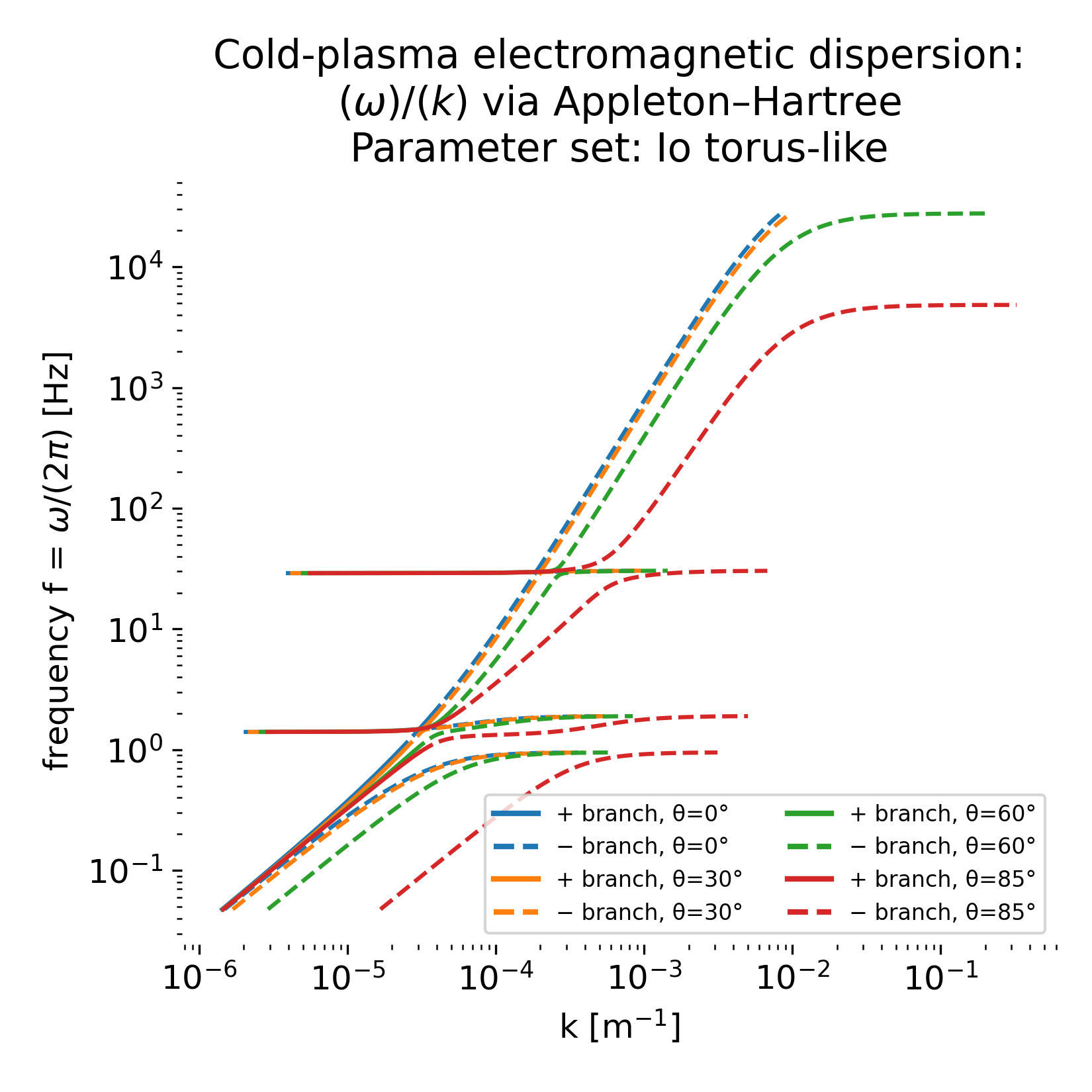
Cold plasma electromagnetic dispersion relation $\omega(k)$ computed from the Appleton–Hartree formalism for an Io plasma torus–like, multi-ion parameter set at Jupiter. Shown are the two electromagnetic branches $n^2_\pm$ for oblique propagation at four angles $\theta$ between $\mathbf{k}$ and $\mathbf{B}_0$. Solid lines denote the plus branch and dashed lines the minus branch, with matching colors indicating identical propagation angles. In contrast to the proton–electron cases, multiple heavy-ion cyclotron frequencies introduce several distinct resonance plateaus and cutoff-related terminations. The resulting step-like structure reflects the strong influence of plasma composition on the cold electromagnetic wave spectrum.

Quasi-neutrality is enforced by taking the electron density equal to the total positive charge density. The model composition is deliberately simplified, but it already captures the essential point: O$^+$ and S$^+$ introduce additional ion cyclotron scales that sit well below the proton cyclotron frequency. Consequently, the dispersion diagram develops multiple distinct resonance plateaus and branch terminations associated with the different ion species.

In the $\omega(k)$ diagram, this appears as a sequence of nearly horizontal segments at characteristic frequencies. These plateaus are the cold-plasma imprint of ion cyclotron resonances of the dominant heavy ions. Because $m_O$ and $m_S$ are much larger than $m_p$, their cyclotron frequencies $\Omega_O = eB_0/m_O$ and $\Omega_S = eB_0/m_S$ are correspondingly smaller, producing resonance structure deep in the low-frequency range. The result is a spectrum that is no longer organized around a single ion cyclotron scale but instead exhibits a multi-step structure reflecting composition.

At higher frequencies, the branches again connect into strongly dispersive electromagnetic behavior, and the angular dependence remains pronounced, as expected for oblique propagation in an anisotropic dielectric medium. The Io torus thus provides a clear demonstration that, even before warm-plasma or kinetic effects are included, the cold electromagnetic dispersion relation already carries direct information about ion composition and magnetospheric environment.

Plasma waves as a bridge between fluid and kinetic theory

Plasma waves form the dynamical backbone of space plasma physics. Their mathematical description naturally interpolates between continuum fluid theory and phase space kinetics. In the next two posts, we will see how this general framework will be specialized to Alfvén and magnetosonic waves and how it can be extended to plasma instabilities, where dispersion relations acquire imaginary components and wave growth replaces simple propagation.

Stay tuned.

Update and code availability: This post and its accompanying Python code were originally drafted in 2020 and archived during the migration of this website to Jekyll and Markdown. In January 2026, I substantially revised and extended the code. The updated and cleaned-up implementation is now available in this new GitHub repositoryꜛ. Please feel free to experiment with it and to share any feedback or suggestions for further improvements.

References and further reading

• Wolfgang Baumjohann and Rudolf A. Treumann, Basic Space Plasma Physics, 1997, Imperial College Press, ISBN: 1-86094-079-X
• Treumann, R. A., Baumjohann, W., Advanced Space Plasma Physics, 1997, Imperial College Press, ISBN: 978-1-86094-026-2
• Stix, T. H., Waves in Plasmas, 1997, American Institute of Physics, ISBN: 978-0883188590
• Francis F. Chen, Introduction to plasma physics and controlled fusion, 2016, Springer, ISBN: 978-3319223087
• Swanson, D. G., Plasma waves, 1989, Academic Press, ISBN: 978-0126789553
• Nicholson, Introduction to Plasma Theory, 1992, Krieger Publishing Company, ISBN: 978-0894646775
• Gary, S. P., Theory of space plasma microinstabilities, 1993, Cambridge University Press, ISBN: 978-0521431675
• Davidson, R. C., Methods in nonlinear plasma theory, 1972, Academic Press, ISBN: 978-0124315365
• Thomas J. M. Boyd & J. J. Sanderson, The Physics of Plasmas, 2003, Cambridge University Press, ISBN: 978-0521459129
• Kivelson, M. G., Russell, C. T. (eds.), Introduction to space physics, 1995, Cambridge University Press, ISBN: 978-0521457149
• Landau, L. D., On the vibrations of the electronic plasma, 1946/1965, Collected Papers of L.D. Landau, Pergamon, Pages 445-460, ISBN 9780080105864