Kinetic plasma theory: From distribution functions to the Vlasov equation

After the single particle description and magnetohydrodynamics (MHD), the kinetic description naturally fills the conceptual gap between the two. Single particle theory follows the exact trajectory of an individual charged particle in prescribed electromagnetic fields. MHD, in contrast, treats the plasma as a conducting fluid and focuses on macroscopic fields, flows, and conserved quantities. The kinetic approach unifies these perspectives. It describes a plasma as a very large ensemble of particles, but without tracking each particle individually. Instead, the fundamental object is a distribution function defined on phase space. This function retains precisely the physics that MHD averages away: Velocity space structure, non Maxwellian populations, temperature anisotropies, drifts, beams, loss cones, weak collisionality, resonances, and wave particle interactions.

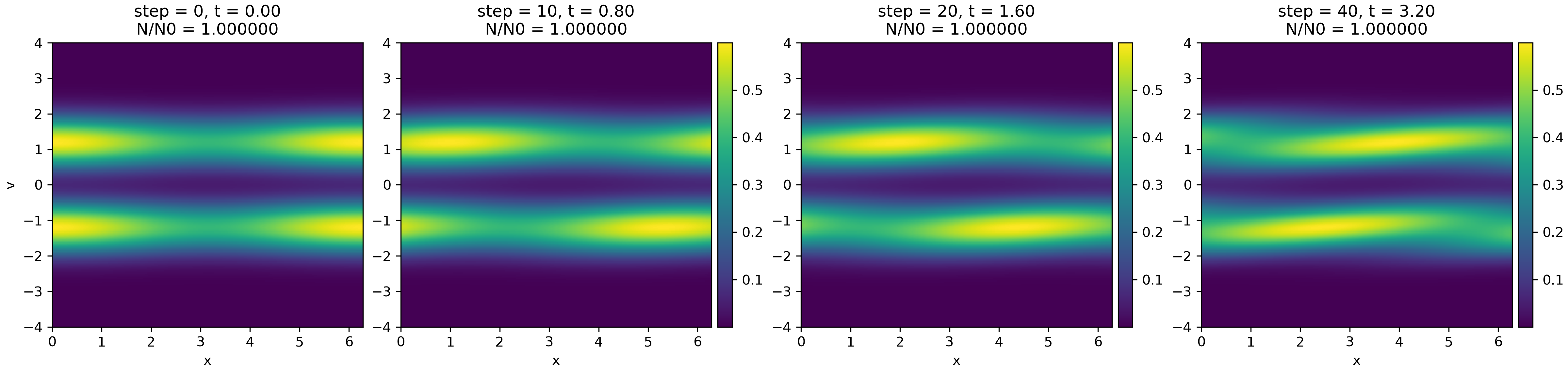
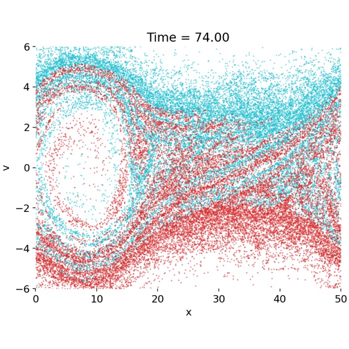
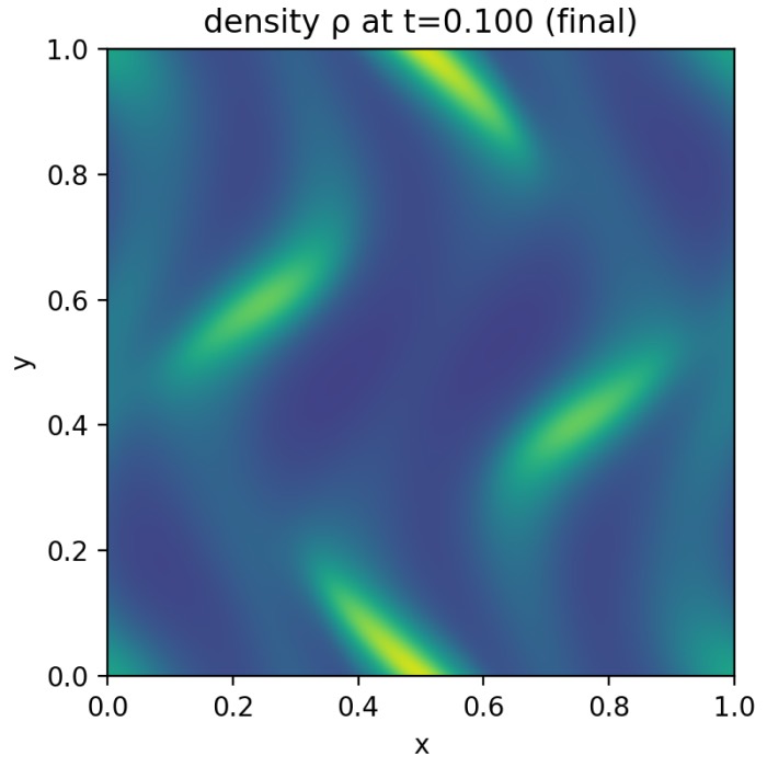
Collisionless Vlasov evolution in one spatial and one velocity dimension. Shown is the phase-space distribution $f(x,v,t)$ for a weakly modulated two-stream initial condition, evolved with a semi-Lagrangian scheme. In the absence of forces and collisions, each velocity slice is advected ballistically in space, leading to phase-space shearing while conserving particle number exactly ($N/N_0=1$). The figure illustrates Liouville’s theorem and the purely advective nature of the Vlasov equation. The Python code to generate this figure is available in this GitHub repositoryꜛ.

In space plasma physics, these effects are not corrections to an otherwise fluid like system. They are often the dominant phenomena. In this post, we explore the foundations of kinetic plasma theory, starting from the definition of the distribution function and leading to the Vlasov equation, which governs its evolution in collisionless plasmas.

Levels of description and the role of kinetic theory

A plasma is a quasineutral ensemble of charged particles with collective behavior. As a many body system, it admits several levels of description that differ in accuracy and complexity.

The most fundamental level is the exact many particle description. One solves Newton’s equations for every particle, coupled self consistently to Maxwell’s equations for the electromagnetic fields. Conceptually this is clean, but analytically intractable and computationally prohibitive for realistic systems. Numerically, this idea is implemented by the particle in cell method, where many real particles are represented by macroparticles, and fields are computed on a grid with full particle field feedback.

At the opposite end lies the fluid description. Here one characterizes the plasma by a small number of macroscopic fields such as density, bulk velocity, pressure, and magnetic field. These quantities obey conservation laws obtained by taking velocity moments of the kinetic equations and closing the hierarchy with additional assumptions. MHD is a particular, strongly closed member of this class.

Between these extremes sits the kinetic description. It replaces the trajectories of individual particles by a distribution function on six dimensional phase space. This approach is rich enough to recover MHD as a limiting case, yet detailed enough to capture deviations from fluid behavior. Structurally, it is the central framework: single particle dynamics is the microscopic limit, MHD is a projection onto low order moments, and kinetic theory provides the controlled link between them.

The distribution function as the fundamental quantity

The distribution function or phase space density $f(\mathbf{x},\mathbf{v},t)$ is defined such that the number of particles in an infinitesimal phase space volume element is

\[dN = f(\mathbf{x},\mathbf{v},t)\, d^3x\, d^3v.\]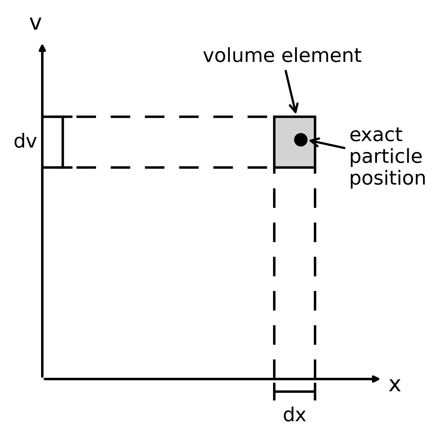

Schematic illustration of phase space in one spatial and one velocity dimension. A particle with exact position $(x,v)$ is represented statistically by a finite phase-space volume element $dx,dv$. The distribution function $f(x,v,t)$ measures the particle density within such elements. In collisionless dynamics governed by the Vlasov equation, phase-space volume is conserved along particle trajectories (Liouville’s theorem): The element may deform as it is advected, but its area remains constant. The Python code to generate this figure is available in this GitHub repositoryꜛ.

Its units therefore read

\[[f] = \frac{1}{\mathrm{m}^3}\frac{1}{(\mathrm{m/s})^3} = \frac{\mathrm{s}^3}{\mathrm{m}^6}.\]

All macroscopic plasma quantities follow from velocity space moments of $f$. The number density is

\[n(\mathbf{x},t) = \int f(\mathbf{x},\mathbf{v},t)\, d^3v.\]

The bulk velocity is

\[\mathbf{u}(\mathbf{x},t) = \frac{1}{n}\int \mathbf{v}\, f(\mathbf{x},\mathbf{v},t)\, d^3v.\]

The pressure tensor is

\[\mathbf{P}(\mathbf{x},t) = m \int (\mathbf{v}-\mathbf{u})(\mathbf{v}-\mathbf{u})\, f(\mathbf{x},\mathbf{v},t)\, d^3v.\]

Only in the isotropic limit does this tensor reduce to a scalar pressure. Already at this level it becomes clear why MHD closures are restrictive: even when density and bulk velocity appear smooth, the velocity space structure encoded in $f$ can be highly non trivial.

Phase space dynamics, Liouville theorem, and the Boltzmann equation

In the absence of collisions, motion in phase space is deterministic. Along a trajectory $(\mathbf{x}(t),\mathbf{v}(t))$, the phase space density is conserved. This statement is formalized by Liouville’s theorem.

The time evolution of phase space for the simple harmonic oscillator. The harmonic oscillator provides a minimal example of Liouville’s theorem: Phase-space elements rotate and deform under Hamiltonian flow while conserving their volume. The Vlasov equation generalizes this geometric picture to collisionless plasmas, where the distribution function is advected in phase space by self-consistent electromagnetic fields. Source: Wikimedia Commons (license: CC BY-SA 3.0).

Introducing the total derivative along a dynamical path,

\[\frac{Df}{Dt} = \frac{\partial f}{\partial t} + \dot{\mathbf{x}}\cdot\nabla f + \dot{\mathbf{v}}\cdot\nabla_{\mathbf{v}} f,\]

and using $\dot{\mathbf{x}}=\mathbf{v}$ and $\dot{\mathbf{v}}=\mathbf{a}=\mathbf{F}/m$, one finds

\[\frac{Df}{Dt} = \frac{\partial f}{\partial t} + \mathbf{v}\cdot\nabla f + \frac{\mathbf{F}}{m}\cdot\nabla_{\mathbf{v}} f.\]

Collisions modify the number of particles in a given phase space volume by scattering particles in and out. This effect is represented by a collision operator, leading to the Boltzmann transport equation

\[\frac{\partial f}{\partial t} + \mathbf{v}\cdot\nabla f + \frac{\mathbf{F}}{m}\cdot\nabla_{\mathbf{v}} f = \left(\frac{\partial f}{\partial t}\right)_{\mathrm{col}}.\]

For a plasma, the relevant force is typically the Lorentz force, with gravity often negligible:

\[\mathbf{F}(\mathbf{x},\mathbf{v},t) = q\big(\mathbf{E}(\mathbf{x},t) + \mathbf{v}\times \mathbf{B}(\mathbf{x},t)\big).\]

The kinetic equation for a plasma species then reads

\[\frac{\partial f}{\partial t} + \mathbf{v}\cdot\nabla f + \frac{q}{m}\big(\mathbf{E} + \mathbf{v}\times \mathbf{B}\big)\cdot\nabla_{\mathbf{v}} f = \left(\frac{\partial f}{\partial t}\right)_{\mathrm{col}}.\]

Together with Maxwell’s equations, this forms a self consistent and extremely general description of plasma dynamics. Its difficulty lies not in conceptual ambiguity but in dimensionality and nonlinearity.

Collision models and their regimes of validity

The collision term encodes irreversibility and relaxation. Its form depends strongly on the physical regime.

For neutral gases with short range interactions, collisions can be treated as discrete two body events, leading to the classical Boltzmann collision integral and, in equilibrium, to the Maxwell Boltzmann distribution.

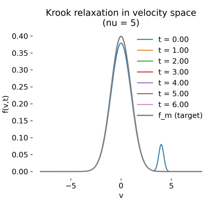
In partially ionized plasmas where collisions with neutrals dominate, a common approximation is a relaxation model of Krook type,

\[\left(\frac{\partial f}{\partial t}\right)_{\mathrm{col}} = \nu_m (f_m - f),\]

where $\nu_m$ is the collision frequency and $f_m$ the neutral distribution. Physically, this represents exponential relaxation toward the neutral background.

In fully ionized plasmas, long range Coulomb interactions dominate. Many small angle deflections accumulate, leading to a Fokker Planck structure, often written schematically as

\[\left(\frac{\partial f}{\partial t}\right)_{\mathrm{col}} = \nabla_{\mathbf{v}}\cdot\big(\mathbf{D}\,\nabla_{\mathbf{v}} f\big),\]

with $\mathbf{D}$ a velocity space diffusion tensor. This is closely related to the Landau collision integral.

The Vlasov equation and collisionless space plasmas

Many space plasmas are sufficiently tenuous that classical collisions are rare. In this limit one sets

\[\left(\frac{\partial f}{\partial t}\right)_{\mathrm{col}} = 0\]

and obtains the Vlasov equation

\[\frac{\partial f}{\partial t} + \mathbf{v}\cdot\nabla f + \frac{q}{m}\big(\mathbf{E} + \mathbf{v}\times \mathbf{B}\big)\cdot\nabla_{\mathbf{v}} f = 0,\]

or compactly

\[\frac{Df}{Dt} = 0.\]

This equation captures a central feature of space plasma physics: non equilibrium distributions are not transient anomalies but long lived states. Relaxation proceeds not through collisions but through wave particle interactions, resonances, instabilities, and phase space mixing. It is precisely here that kinetic theory goes beyond any fluid description.

Standard forms of the distribution function

Several standard forms of the distribution function are widely used to model different plasma regimes and phenomena.

Maxwell Boltzmann distribution

In thermal equilibrium the distribution is isotropic and Maxwellian,

\[f(\mathbf{v}) = n\left(\frac{m}{2\pi k_B T}\right)^{3/2}\exp\!\left(-\frac{m v^2}{2k_B T}\right).\]

The temperature sets a characteristic thermal speed scale,

\[v_{\mathrm{th}} \sim \sqrt{\frac{2k_B T}{m}},\]

up to convention dependent numerical factors.

Drifting Maxwellian

If the plasma possesses a bulk flow $\mathbf{v}_0$, the distribution is shifted in velocity space,

\[f(\mathbf{v}) = n\left(\frac{m}{2\pi k_B T}\right)^{3/2}\exp\!\left(-\frac{m(\mathbf{v}-\mathbf{v}_0)^2}{2k_B T}\right).\]

This is the kinetic counterpart of the MHD flow velocity.

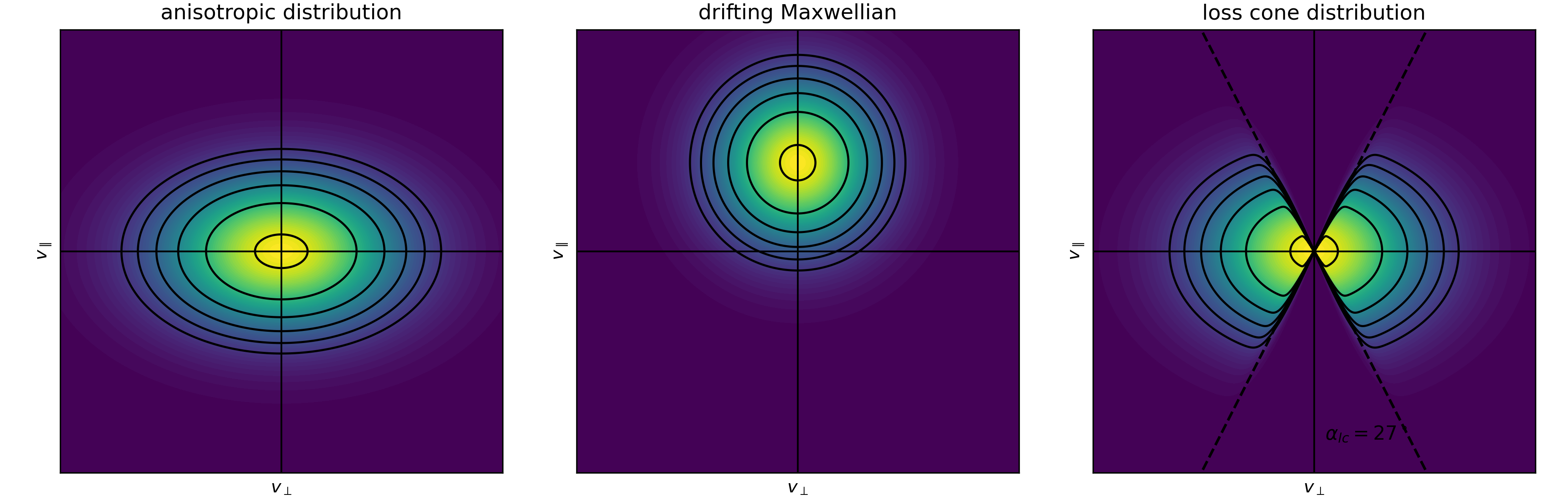
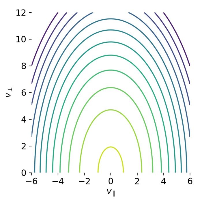
Representative velocity-space distributions in a magnetized plasma, shown in the $(v_\perp, v_\parallel)$ plane. Left: anisotropic bi-Maxwellian with different perpendicular and parallel temperatures $(T_\perp \neq T_\parallel)$, producing elliptical contours. Center: drifting Maxwellian, shifted along the parallel velocity direction by a bulk drift $u_\parallel$. Right: loss-cone distribution, where particles with small pitch angles are depleted due to escape along magnetic field lines; dashed lines indicate the loss-cone boundary $\alpha_{lc}$. Contours denote constant values of the distribution function. The Python code to generate this figure is available in this GitHub repositoryꜛ.

Bi Maxwellian and temperature anisotropy

A magnetic field breaks isotropy by distinguishing motion parallel and perpendicular to $\mathbf{B}$. A common model is the bi Maxwellian,

\[f(v_\perp,v_\parallel) \propto \exp\!\left(-\frac{m v_\perp^2}{2k_B T_\perp} - \frac{m v_\parallel^2}{2k_B T_\parallel}\right).\]

The distribution is gyrotropic, independent of the gyrophase angle, but anisotropic in temperature. Even this simplest magnetized distribution already implies a pressure tensor rather than a scalar pressure.

Loss cones

In magnetospheric systems, particles with certain pitch angles stream along field lines into the atmosphere and are lost. The resulting depletion in phase space produces a loss cone. This is a purely kinetic effect arising from the geometry of magnetic field lines and particle invariants.

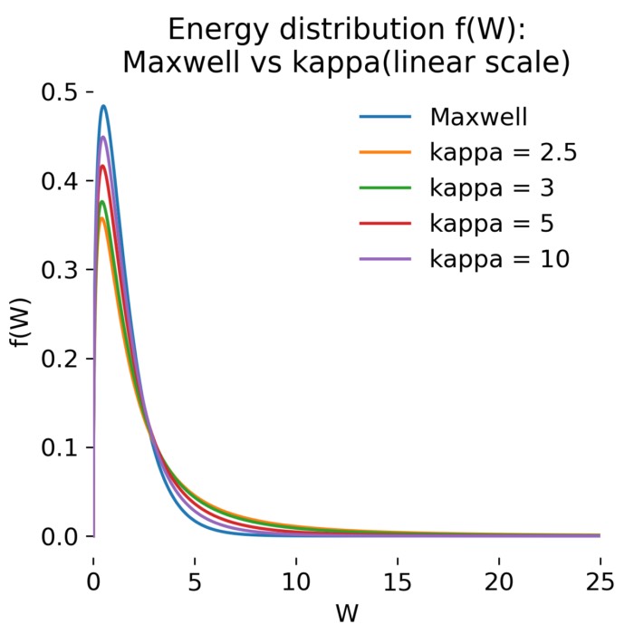
Kappa distributions and suprathermal tails

Observed space plasma distributions often exhibit high energy tails that fall off more slowly than a Maxwellian. A widely used phenomenological model is the kappa distribution. In energy space one typical form is

\[f_\kappa(W) = n \left( \frac{m}{2\pi \kappa W_0} \right)^{3/2} \frac{\Gamma(\kappa+1)}{\Gamma(\kappa-\frac{1}{2})} \left(1+\frac{W}{\kappa W_0}\right)^{-(\kappa+1)}.\]

As $\kappa \to \infty$, the Maxwellian is recovered. The kappa distribution is not a derivation of a specific mechanism, but an efficient way to parameterize the persistent presence of suprathermal particle populations, which are invisible in a purely fluid description.

How distribution functions are measured in space

Experimentally, the distribution function is usually inferred indirectly via the differential particle flux $J$. For an isotropic velocity element,

\[d^3v = v^2\, dv\, d\Omega,\]

with $d\Omega$ the solid angle. The flux through a detector area introduces an additional factor of $v$. Expressing the distribution in terms of energy $W=\frac{1}{2}mv^2$ with $dW=mv\,dv$, one finds

\[J(W,\alpha,\mathbf{x}) = \frac{v^2}{m}\, f(v_\perp,v_\parallel,\mathbf{x}).\]

The measured quantity thus carries units of particles per area, time, energy, and solid angle. This explains why spacecraft data are typically presented in terms of flux rather than $f$ itself.

From kinetic theory to MHD via moments

The connection to MHD is obtained by taking velocity moments of the kinetic equation.

The zeroth moment yields the continuity equation,

\[\frac{\partial n}{\partial t} + \nabla\cdot(n\mathbf{u}) = 0,\]

in the collisionless, source free case.

The first moment gives the momentum equation,

\[mn\left(\frac{\partial \mathbf{u}}{\partial t} + \mathbf{u}\cdot\nabla \mathbf{u}\right) = qn(\mathbf{E}+\mathbf{u}\times\mathbf{B}) - \nabla\cdot \mathbf{P}.\]

At this point the hierarchy must be closed. Replacing the pressure tensor by a scalar pressure and prescribing an equation of state is precisely the step that turns kinetic theory into MHD. In weakly collisional, magnetized plasmas, this closure is often only marginally justified.

What kinetic theory reveals beyond MHD

The differences between kinetic and fluid descriptions are structural, not cosmetic. Kinetic theory captures instabilities driven by velocity space gradients, Landau damping and resonant energy transfer without collisions, phase space filamentation, and long lived non equilibrium states. MHD, by contrast, excels at describing large scale field topology, global flows, and long wavelength dynamics.

The correct perspective is therefore not kinetic theory versus MHD, but hierarchy and projection. MHD is a low moment projection of kinetic dynamics. Kinetic theory specifies when this projection is valid and what physics is lost when it is applied outside its regime.

Conclusion

In space plasma physics, the collisionless limit is not a technical simplification but the natural state of many systems. The Vlasov Maxwell framework is therefore not optional. It is the minimal theory that treats electromagnetic fields self consistently while retaining the full velocity space structure of the particle population. MHD remains indispensable for global, large scale problems. Kinetic theory, however, is where one understands how microscopic particle dynamics generates collective fields, and how those fields in turn sculpt the phase space distribution. Any serious attempt to understand space plasmas must ultimately return to the distribution function $f(\mathbf{x},\mathbf{v},t)$.

Update and code availability: This post and its accompanying Python code were originally drafted in 2020 and archived during the migration of this website to Jekyll and Markdown. In January 2026, I substantially revised and extended the code. The updated and cleaned-up implementation is now available in this new GitHub repositoryꜛ. Please feel free to experiment with it and to share any feedback or suggestions for further improvements.

References and further reading

• Wolfgang Baumjohann and Rudolf A. Treumann, Basic Space Plasma Physics, 1997, Imperial College Press, ISBN: 1-86094-079-X
• Treumann, R. A., Baumjohann, W., Advanced Space Plasma Physics, 1997, Imperial College Press, ISBN: 978-1-86094-026-2
• Donald A. Gurnett, Amitava Bhattacharjee, Introduction to plasma physics with space and laboratory applications, 2005, Cambridge University Press, ISBN: 978-7301245491
• Francis F. Chen, Introduction to plasma physics and controlled fusion, 2016, Springer, ISBN: 978-3319223087
• R. C. Davidson, Methods in nonlinear plasma theory, 1972, Academic Press, ISBN: 978-0122054501