Bi-Maxwellian distributions and anisotropic pressure

September 11, 2020 January 23, 2026 9 minute read see also comments

In many space and laboratory plasmas, the assumption of an isotropic thermal equilibrium is not justified. In particular, in magnetized and weakly collisional plasmas, the presence of a strong magnetic field separates the dynamics parallel and perpendicular to the field. Particles move freely along magnetic field lines, while their perpendicular motion is constrained by gyromotion. As a result, the kinetic energy associated with parallel and perpendicular motion generally evolves differently.

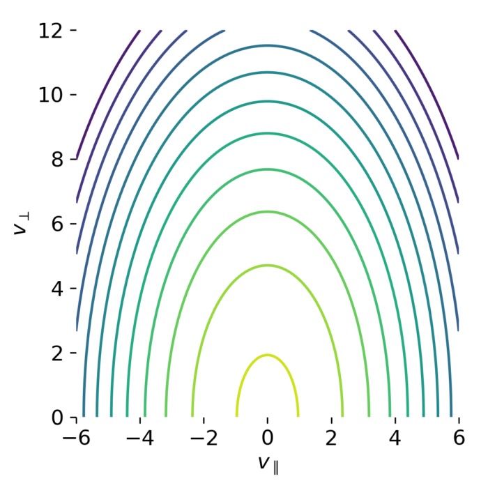
$Snippet of velocity-space contour plots of bi-Maxwellian distributions for different temperature anisotropies $T_\perp / T_\parallel$.$
Snippet of velocity-space contour plots of bi-Maxwellian distributions for different temperature anisotropies $T_\perp / T_\parallel$. The elongation of the contours directly reflects the imposed anisotropy. In this post, we explore how such anisotropic velocity distributions lead to anisotropic pressure components.

From a kinetic perspective, this naturally leads to velocity distributions that cannot be described by a single scalar temperature. Instead, two independent temperatures are required: A parallel temperature $T_\parallel$ and a perpendicular temperature $T_\perp$. The simplest self-consistent model capturing this situation is the bi-Maxwellian distribution.

The purpose of the numerical example provided in this post is to make this anisotropy explicit in velocity space and to demonstrate how it translates directly into anisotropic pressure components. At the same time, the bi-Maxwellian serves as a canonical reference case: Its moments can be computed analytically, making it ideal for validating numerical integration and for illustrating the limitations of isotropic fluid closures.

Physical model: Bi-Maxwellian velocity distribution

We consider a homogeneous, stationary, magnetized plasma population without bulk drift. The velocity distribution function is taken to be a bi-Maxwellian of the form

\[f(v_\perp, v_\parallel) = \frac{n}{(2\pi)^{3/2} v_\perp^2 v_\parallel} \exp\!\left( -\frac{v_\perp^2}{2 v_\perp^2} -\frac{v_\parallel^2}{2 v_\parallel^2} \right),\]

where $v_\perp$ and $v_\parallel$ denote the particle velocities perpendicular and parallel to the magnetic field, respectively. The thermal velocities are related to the corresponding temperatures by

\[v_\perp^2 = \frac{k_B T_\perp}{m}, \quad v_\parallel^2 = \frac{k_B T_\parallel}{m}.\]

The distribution is gyrotropic and depends only on the magnitudes of $v_\perp$ and $v_\parallel$, not on the gyrophase. Physically, this describes a plasma that is homogeneous and time independent, but whose microscopic energy content is distributed anisotropically with respect to the magnetic field direction.

Pressure moments and anisotropy

From a kinetic point of view, pressure components are defined as second-order central velocity moments of the distribution function. For a bi-Maxwellian distribution, the parallel and perpendicular pressure components are given by

\[P_\parallel = m \int (v_\parallel - u_\parallel)^2 f \, d^3v,\] \[P_\perp = \frac{m}{2} \int v_\perp^2 f \, d^3v,\]

where the factor $1/2$ accounts for the two perpendicular degrees of freedom. Since the distribution is drift-free, $u_\parallel = 0$.

For the bi-Maxwellian, these integrals can be evaluated analytically, yielding

\[P_\parallel = n k_B T_\parallel, \quad P_\perp = n k_B T_\perp.\]

It follows immediately that

\[\frac{P_\perp}{P_\parallel} = \frac{T_\perp}{T_\parallel}.\]

This relation is elementary but physically fundamental. It shows that anisotropic pressure is a direct and unavoidable consequence of anisotropic velocity distributions, without invoking any collective dynamics or time evolution.

Numerical realization

Numerically, the distribution function is discretized on a two-dimensional velocity grid in $(v_\parallel, v_\perp)$. The grid is chosen symmetric about $v_\parallel = 0$ and extends sufficiently far in velocity space to resolve the exponential decay of the distribution.

The numerical procedure consists of the following steps:

definition of a Cartesian grid in $(v_\parallel, v_\perp)$
evaluation of the bi-Maxwellian distribution for prescribed values of $T_\perp$ and $T_\parallel$
numerical quadrature of the pressure moments using direct summation
systematic variation of the temperature ratio $T_\perp/T_\parallel$ over several orders of magnitude
comparison of numerically computed pressure ratios with the analytic reference relation

No time dependence or self-consistent fields are included. The example is deliberately static, designed to isolate the mapping from velocity-space structure to macroscopic pressure components.

We begin again by importing necessary libraries and setting plotting parameters.

import numpy as np
import matplotlib.pyplot as plt

# remove spines right and top for better aesthetics:
plt.rcParams['axes.spines.right'] = False
plt.rcParams['axes.spines.top'] = False
plt.rcParams['axes.spines.left'] = False
plt.rcParams['axes.spines.bottom'] = False
plt.rcParams.update({'font.size': 12})

The first step is to define the bi-Maxwellian distribution function:

def bi_maxwellian(v_perp, v_par, n=1.0, T_perp=1.0, T_par=1.0, m=1.0, kB=1.0, u_par=0.0):
    pref = n * (m / (2.0 * np.pi * kB * T_perp)) * np.sqrt(m / (2.0 * np.pi * kB * T_par))
    expo = np.exp(
        -(m * v_perp**2) / (2.0 * kB * T_perp)
        -(m * (v_par - u_par) ** 2) / (2.0 * kB * T_par)
    )
    return pref * expo

Next, we need a function to compute the relevant velocity moments and pressures from the discretized distribution function:

def compute_moments_pressure(vperp_grid, vpar_grid, f, m=1.0, u_par=0.0):
    dvperp = vperp_grid[1] - vperp_grid[0]
    dvpar = vpar_grid[1] - vpar_grid[0]

    VPERP, VPAR = np.meshgrid(vperp_grid, vpar_grid, indexing="xy")
    weight = 2.0 * np.pi * VPERP * dvperp * dvpar  # d^3v weights

    n = np.sum(f * weight)
    P_par = m * np.sum(((VPAR - u_par) ** 2) * f * weight)
    P_perp = 0.5 * m * np.sum((VPERP**2) * f * weight)

    return n, P_perp, P_par

and a helper function to create suitable velocity grids:

def make_velocity_grids(T_perp, T_par, m=1.0, kB=1.0, n_sigma=6.0, Nvperp=400, Nvpar=600):
    vth_perp = np.sqrt(kB * T_perp / m)
    vth_par = np.sqrt(kB * T_par / m)

    vperp_max = n_sigma * vth_perp
    vpar_max = n_sigma * vth_par

    vperp = np.linspace(0.0, vperp_max, Nvperp)
    vpar = np.linspace(-vpar_max, vpar_max, Nvpar)
    return vperp, vpar

To run the demo, we set some example parameters and define the range of anisotropy ratios to explore:

# some demo parameters:
m = 1.0         # particle mass
kB = 1.0        # Boltzmann constant (here set to 1 for convenience)
n0 = 1.0        # number density
u_par = 0.0     # parallel bulk velocity

# base parallel temperature and a sweep over anisotropy ratios:
T_par0 = 1.0
anisotropy_list = [0.25, 0.5, 1.0, 2.0, 4.0]  # T_perp / T_par

# for the pressure-ratio curve:
anisotropy_curve = np.logspace(-1, 1, 17)  # 0.1 ... 10

Our first plot shows contour lines of the bi-Maxwellian distribution in the $(v_\parallel, v_\perp)$ plane for selected anisotropy ratios:

# plot 1: contour plots for selected anisotropies:
# create a row of panels for f(v_par, v_perp) contours.
fig, axes = plt.subplots(1, len(anisotropy_list), 
                         figsize=(4.2 * len(anisotropy_list), 4), 
                         sharey=True)

for ax, a in zip(axes, anisotropy_list):
    T_perp0 = a * T_par0
    vperp, vpar = make_velocity_grids(T_perp0, T_par0, m=m, kB=kB, n_sigma=6.0, Nvperp=280, Nvpar=420)

    VPERP, VPAR = np.meshgrid(vperp, vpar, indexing="xy")
    f = bi_maxwellian(VPERP, VPAR, n=n0, T_perp=T_perp0, T_par=T_par0, m=m, kB=kB, u_par=u_par)

    # Use log contours for dynamic range (avoid log(0) by adding tiny floor)
    f_floor = np.max(f) * 1e-12
    f_log = np.log10(f + f_floor)

    cs = ax.contour(VPAR, VPERP, f_log, levels=12)
    ax.set_title(rf"$T_\perp/T_\parallel = {a:g}$")
    ax.set_xlabel(r"$v_\parallel$")
    if ax is axes[0]:
        ax.set_ylabel(r"$v_\perp$")

plt.tight_layout()
plt.savefig("bi_maxwellian_anisotropy_contours.png", dpi=300)
plt.close()

And the second plot compares the numerically computed pressure ratios with the analytic reference relation:

# plot 2: pressure ratio vs temperature ratio:
ratios_T = []
ratios_P = []
densities = []

for a in anisotropy_curve:
    T_perp0 = a * T_par0
    vperp, vpar = make_velocity_grids(T_perp0, T_par0, m=m, kB=kB, n_sigma=7.0, Nvperp=400, Nvpar=600)

    VPERP, VPAR = np.meshgrid(vperp, vpar, indexing="xy")
    f = bi_maxwellian(VPERP, VPAR, n=n0, T_perp=T_perp0, T_par=T_par0, m=m, kB=kB, u_par=u_par)

    n_calc, P_perp, P_par = compute_moments_pressure(vperp, vpar, f, m=m, u_par=u_par)

    ratios_T.append(a)
    ratios_P.append(P_perp / P_par)
    densities.append(n_calc)

ratios_T = np.array(ratios_T)
ratios_P = np.array(ratios_P)
densities = np.array(densities)

plt.figure(figsize=(6.2, 4.8))
plt.plot(ratios_T, ratios_P, marker="o", label=r"numerical: $P_\perp/P_\parallel$")
plt.plot(ratios_T, ratios_T, linestyle="--", label=r"reference: $P_\perp/P_\parallel = T_\perp/T_\parallel$")
plt.xscale("log")
plt.yscale("log")
plt.xlabel(r"$T_\perp/T_\parallel$")
plt.ylabel(r"$P_\perp/P_\parallel$")
plt.title("Bi-Maxwellian anisotropy: Pressure ratio\ntracks temperature ratio")
plt.grid(True, which="both", alpha=0.3)
plt.legend(frameon=False)
plt.tight_layout()
plt.savefig("bi_maxwellian_pressure_vs_temperature_ratio.png", dpi=300)
plt.close()

Discussion of the results

In the following, we discuss the two key results from our numerical calculations above.

Pressure ratio versus temperature ratio

The first result plot shows the ratio $P_\perp / P_\parallel$ as a function of the imposed temperature ratio $T_\perp / T_\parallel$ on logarithmic axes. Over the entire explored parameter range, the numerical data lie exactly on the reference line

\[\frac{P_\perp}{P_\parallel} = \frac{T_\perp}{T_\parallel}.\]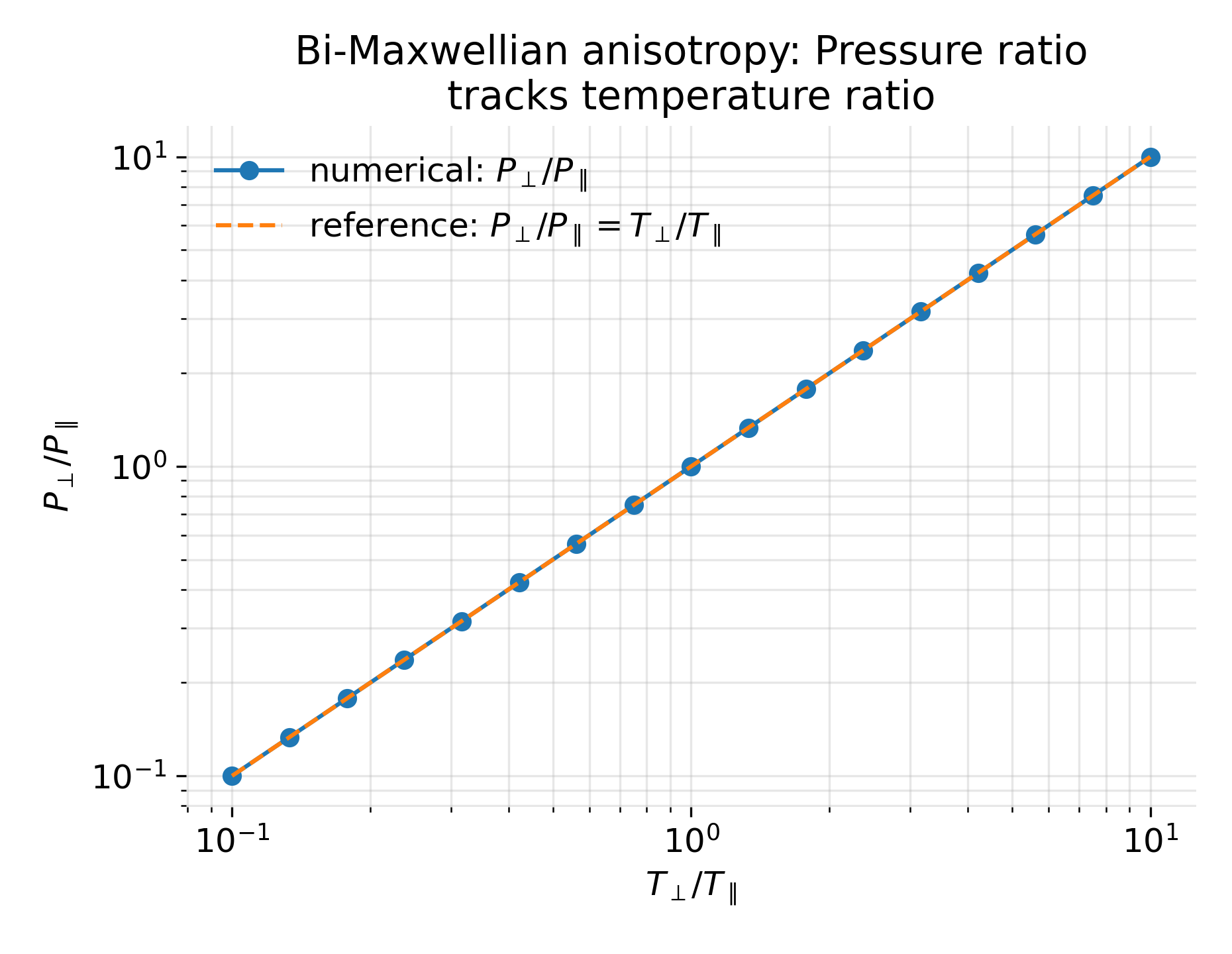

Pressure anisotropy in a bi-Maxwellian plasma. Numerically computed ratio $P_\perp / P_\parallel$ as a function of the imposed temperature ratio $T_\perp / T_\parallel$ for a gyrotropic bi-Maxwellian distribution. Blue markers show the pressure ratio obtained from direct numerical integration of the velocity moments, while the dashed line indicates the analytic relation $P_\perp / P_\parallel = T_\perp / T_\parallel$. The perfect agreement over several orders of magnitude confirms that pressure anisotropy follows directly from velocity-space anisotropy.

This confirms that the numerical integration correctly reproduces the analytic velocity moments of the bi-Maxwellian distribution. At the same time, it illustrates that pressure anisotropy is not an emergent or approximate effect in this case, but follows directly from the structure of the distribution function.

The plot thus serves a dual role: It validates the numerical method and provides a clear visual statement of the kinetic origin of anisotropic pressure.

Velocity-space contour plots

The second result plot shows contour lines of the distribution function in the $(v_\parallel, v_\perp)$ plane for several values of $T_\perp/T_\parallel$.

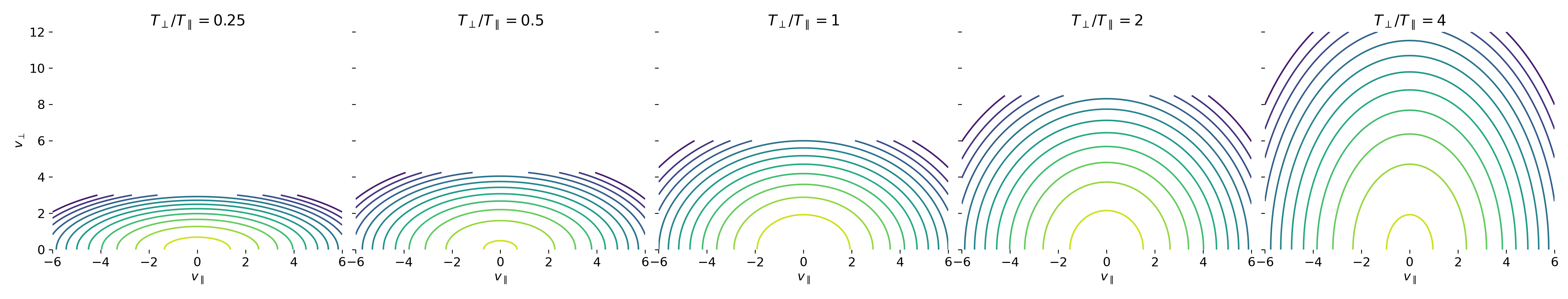
Velocity-space structure of bi-Maxwellian distributions. Contour plots of the bi-Maxwellian distribution function $f(v_\parallel, v_\perp)$ for different temperature ratios $T_\perp / T_\parallel$. The contours form ellipses whose axis ratio is set by $\sqrt{T_\perp / T_\parallel}$, illustrating how anisotropic temperatures correspond to anisotropic velocity-space geometry. For $T_\perp / T_\parallel < 1$ the distribution is elongated parallel to the magnetic field, while for $T_\perp / T_\parallel > 1$ it is elongated in the perpendicular direction.

For $T_\perp/T_\parallel < 1$, the contours are elongated along the parallel direction. The distribution is narrow in $v_\perp$ and broad in $v_\parallel$. For $T_\perp/T_\parallel = 1$, the contours become isotropic, corresponding to an ordinary Maxwellian. For $T_\perp/T_\parallel > 1$, the elongation shifts to the perpendicular direction.

Mathematically, these contours satisfy

\[\frac{v_\perp^2}{T_\perp} + \frac{v_\parallel^2}{T_\parallel} = \text{const},\]

that is, ellipses whose axis ratio is set by $\sqrt{T_\perp/T_\parallel}$. The plots therefore provide a direct geometric visualization of kinetic anisotropy in velocity space.

Physical interpretation

In space plasmas, pressure anisotropy is the rule rather than the exception. In the solar wind, planetary magnetospheres, and magnetosheaths, collision times are often much longer than dynamical timescales. As a result, particle distributions retain memory of adiabatic invariants, most notably the magnetic moment. Variations in magnetic field strength then naturally lead to different evolutions of $T_\perp$ and $T_\parallel$.

Such anisotropic pressure states form the basis of many kinetic instabilities, including the mirror, firehose, and ion-cyclotron instabilities. These processes play a central role in regulating temperature anisotropy and mediating energy transfer in collisionless plasmas. None of these effects can be captured by fluid models that assume a scalar pressure.

The presented example illustrates, in the simplest possible setting, how anisotropic pressure tensors arise directly from velocity-space structure. It therefore provides a conceptual bridge between full kinetic theory and anisotropic fluid or MHD descriptions used in space physics.

Conclusion

By constructing and analyzing bi-Maxwellian velocity distributions, the example in this post demonstrates explicitly how anisotropic pressure emerges from anisotropic kinetic structure. The numerical results reproduce the known analytic relations while providing an intuitive geometric interpretation in velocity space.

More broadly, the example highlights what is retained and what is lost when reducing kinetic theory to fluid models. While fluid descriptions capture averaged quantities, they necessarily discard information about velocity-space geometry that can be dynamically decisive in weakly collisional, magnetized plasmas.

As such, this static and analytically controlled construction serves as a clean starting point for understanding pressure anisotropy, kinetic instabilities, and the limitations of isotropic closures in space plasma physics.

Update and code availability: This post and its accompanying Python code were originally drafted in 2020 and archived during the migration of this website to Jekyll and Markdown. In January 2026, I substantially revised and extended the code. The updated and cleaned-up implementation is now available in this new GitHub repositoryꜛ. Please feel free to experiment with it and to share any feedback or suggestions for further improvements.

References and further reading

Wolfgang Baumjohann and Rudolf A. Treumann, Basic Space Plasma Physics, 1997, Imperial College Press, ISBN: 1-86094-079-X
Treumann, R. A., Baumjohann, W., Advanced Space Plasma Physics, 1997, Imperial College Press, ISBN: 978-1-86094-026-2
Donald A. Gurnett, Amitava Bhattacharjee, Introduction to plasma physics with space and laboratory applications, 2005, Cambridge University Press, ISBN: 978-7301245491
Francis F. Chen, Introduction to plasma physics and controlled fusion, 2016, Springer, ISBN: 978-3319223087
R. C. Davidson, Methods in nonlinear plasma theory, 1972, Academic Press, ISBN: 978-0122054501