Kappa versus Maxwell distributions: Suprathermal tails in collisionless plasmas

September 11, 2020 January 23, 2026 10 minute read see also comments

A central assumption underlying many fluid and kinetic plasma models is that particle velocity distributions relax toward a Maxwellian form. This assumption is well justified in collisional environments, where frequent particle–particle interactions efficiently thermalize the distribution. In large parts of space physics, however, plasmas are weakly collisional or effectively collisionless. Under these conditions, the Maxwellian assumption often fails.

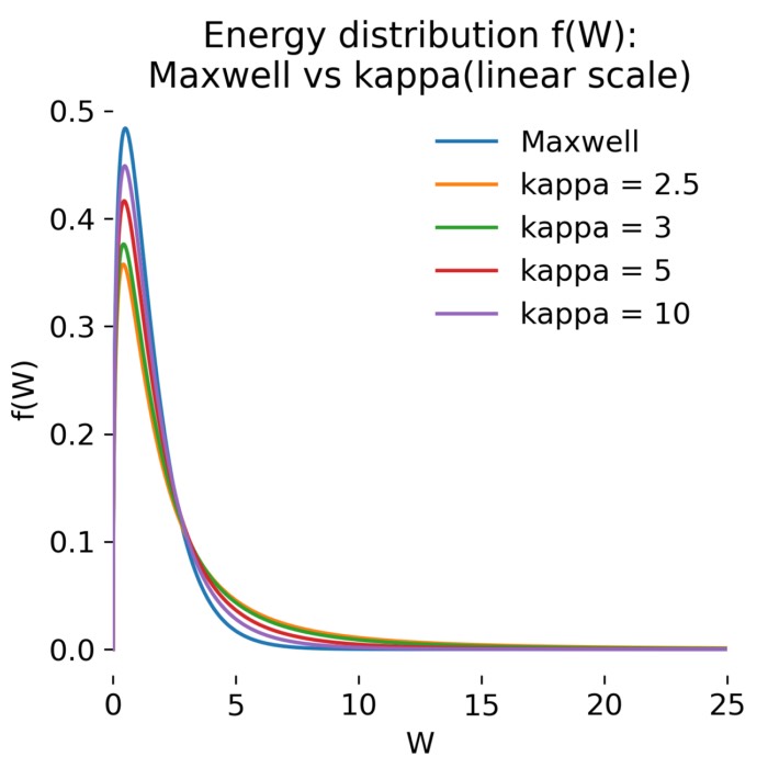
Kappa and Maxwellian energy distributions on a linear scale. In this post, we compare these two distribution functions to highlight the emergence of suprathermal tails in kappa distributions.

Measurements in the solar wind, planetary magnetospheres, and heliospheric boundary regions consistently reveal particle distributions with pronounced suprathermal tails. These high-energy populations decay much more slowly than the exponential tails predicted by Maxwellian statistics. A widely used phenomenological model to describe such distributions is the kappa distribution, which interpolates between a thermal core and a power-law tail.

The purpose of the numerical example presented in this post is to compare Maxwellian and kappa energy distributions in a controlled setting, to visualize the emergence of suprathermal tails, and to quantify their impact on high-energy particle populations. This example complements our earlier demonstrations by highlighting a purely kinetic effect that cannot be captured by fluid models.

Physical model: Energy distributions

We work in energy space and consider isotropic distributions expressed as functions of the kinetic energy

\[W = \frac{1}{2} m v^2.\]

For a three-dimensional Maxwellian velocity distribution, the corresponding energy distribution takes the form

\[f_M(W) \propto W^{1/2} \exp\!\left(-\frac{W}{k_B T}\right),\]

where $T$ is the temperature and $k_B T$ sets the characteristic energy scale. The exponential decay implies that the probability of finding particles at energies much larger than $k_B T$ is extremely small.

The kappa distribution modifies this behavior by replacing the exponential tail with a power-law decay,

\[f_\kappa(W) \propto W^{1/2} \left(1 + \frac{W}{\kappa W_0}\right)^{-(\kappa+1)},\]

where $\kappa$ is a dimensionless parameter controlling the slope of the suprathermal tail and $W_0$ is an energy scale analogous to $k_B T$. For large $\kappa$, the kappa distribution approaches the Maxwellian form, while for small $\kappa$ the tail becomes increasingly pronounced.

Both distributions are normalized such that

\[\int_0^\infty f(W)\,dW = 1.\]

Numerical realization

Numerically, both distributions are evaluated on a one-dimensional energy grid $W \ge 0$ extending over several decades in energy. The grid is chosen sufficiently fine to resolve both the thermal core and the slowly decaying suprathermal tails of the kappa distribution.

The numerical procedure consists of the following steps:

construction of an energy grid $W \in [0, W_{\max}]$
evaluation of the unnormalized Maxwellian and kappa energy distributions
numerical normalization using direct quadrature
comparison of distributions on linear and logarithmic scales
computation of the fraction of particles above a given threshold energy $F(W > W_c) = \int_{W_c}^\infty f(W)\,dW$

The threshold energy $W_c$ is varied to probe the population of suprathermal particles. All integrals are computed numerically using the trapezoidal rule. No time dependence or self-consistent fields are included; the example is static and designed to isolate the statistical properties of the distributions.

So, let’s implement this in Python. We start with some standard imports and plotting configuration:

import numpy as np
import matplotlib.pyplot as plt

# remove spines right and top for better aesthetics:
plt.rcParams['axes.spines.right'] = False
plt.rcParams['axes.spines.top'] = False
plt.rcParams['axes.spines.left'] = False
plt.rcParams['axes.spines.bottom'] = False
plt.rcParams.update({'font.size': 12})

First, we define a function, that normalizes a PDF defined on a 1D grid using the trapezoidal rule:

def normalize_on_grid(W: np.ndarray, f_unnorm: np.ndarray) -> np.ndarray:
    Z = np.trapezoid(f_unnorm, W)
    if Z <= 0 or not np.isfinite(Z):
        raise ValueError("Normalization failed: nonpositive or nonfinite integral.")
    return f_unnorm / Z

We then define the Maxwellian and kappa energy distribution functions:

def maxwell_energy_pdf(W: np.ndarray, kT: float) -> np.ndarray:
    W = np.asarray(W)
    f = np.zeros_like(W, dtype=float)
    mask = W >= 0
    f[mask] = np.sqrt(W[mask]) * np.exp(-W[mask] / kT)
    return f

def kappa_energy_pdf(W: np.ndarray, kappa: float, W0: float) -> np.ndarray:
    if kappa <= 1.5:
        # For many kappa conventions, moments can diverge for small kappa.
        # We keep a conservative guardrail.
        raise ValueError("Choose kappa > 1.5 for a well behaved demonstration.")
    W = np.asarray(W)
    f = np.zeros_like(W, dtype=float)
    mask = W >= 0
    f[mask] = np.sqrt(W[mask]) * (1.0 + W[mask] / (kappa * W0)) ** (-(kappa + 1.0))
    return f

Another helper function computes the tail fraction above a threshold energy:

def tail_fraction(W: np.ndarray, f: np.ndarray, Wc: float) -> float:
    if Wc <= W[0]:
        return 1.0
    if Wc >= W[-1]:
        return 0.0
    idx = np.searchsorted(W, Wc, side="left")
    return float(np.trapezoid(f[idx:], W[idx:]))

Now, let’s set up the parameters for our numerical example and compute the distributions:

kT = 1.0          # energy unit for Maxwellian
kappa_list = [2.5, 3.0, 5.0, 10.0]  # compare several kappa values
W0 = 1.0          # energy scale for kappa distribution
Wmax = 80.0       # max energy shown
NW = 20000        # resolution in W
Wc_values = [3.0, 5.0, 10.0, 20.0]  # thresholds for tail fractions

# energy grid. Start slightly above 0 to avoid sqrt singular visuals:
W = np.linspace(0.0, Wmax, NW)

# compute PDFs:
fM = normalize_on_grid(W, maxwell_energy_pdf(W, kT=kT))

fk_dict = {}
for kap in kappa_list:
    fk = normalize_on_grid(W, kappa_energy_pdf(W, kappa=kap, W0=W0))
    fk_dict[kap] = fk

We can now create the plots and compute the tail fractions. The first plot shows the distributions on a linear scale:

plt.figure(figsize=(6, 4.5))
plt.plot(W, fM, label="Maxwell")
for kap in kappa_list:
    plt.plot(W, fk_dict[kap], label=f"kappa = {kap:g}")
plt.xlim(0, min(Wmax, 25.0))
plt.xlabel("W")
plt.ylabel("f(W)")
plt.title("Energy distribution f(W): Maxwell vs kappa\n(linear scale)")
plt.legend(frameon=False)
plt.tight_layout()
plt.savefig("kappa_vs_maxwell_linear.png", dpi=300)
plt.close()

The second plot uses a logarithmic scale to highlight the suprathermal tails:

plt.figure(figsize=(6, 4.5))
plt.semilogy(W, fM, label="Maxwell")
for kap in kappa_list:
    plt.semilogy(W, fk_dict[kap], label=f"kappa = {kap:g}")
plt.xlim(0, Wmax)
plt.ylim(1e-12, None)
plt.xlabel("W")
plt.ylabel("f(W) (log)")
plt.title("Energy distribution f(W): Suprathermal tails\n(log scale)")
for Wc in Wc_values:
    plt.axvline(Wc, linewidth=1.0, alpha=0.5)
plt.legend(frameon=False, loc="upper right")
plt.tight_layout()
plt.savefig("kappa_vs_maxwell_log.png", dpi=300)
plt.close()

As an additional quantitative measure, we compute and print the tail fractions above selected threshold energies:

print("\nTail fractions F(W > Wc) for selected thresholds")
print(f"Grid: W in [0, {Wmax}] with NW={NW}")
print(f"Maxwell parameter: kT={kT}")
print(f"Kappa parameters: W0={W0}, kappa in {kappa_list}")
print("")
header = "Wc".ljust(8) + "Maxwell".rjust(14)
for kap in kappa_list:
    header += f"  kappa={kap:g}".rjust(14)
print(header)
print("-" * len(header))

for Wc in Wc_values:
    row = f"{Wc:>6.2f}  "
    row += f"{tail_fraction(W, fM, Wc):>12.6e}  "
    for kap in kappa_list:
        row += f"{tail_fraction(W, fk_dict[kap], Wc):>12.6e}  "
    print(row)

And finally, we plot the tail fraction curves as a function of the threshold energy:

Wc_grid = np.linspace(0.0, Wmax, 600)
FM_tail = np.array([tail_fraction(W, fM, wc) for wc in Wc_grid])

plt.figure(figsize=(6, 4.5))
plt.semilogy(Wc_grid, FM_tail, label="Maxwell")
for kap in kappa_list:
    Fk_tail = np.array([tail_fraction(W, fk_dict[kap], wc) for wc in Wc_grid])
    plt.semilogy(Wc_grid, Fk_tail, label=f"kappa = {kap:g}")
plt.ylim(1e-12, 1.0)
plt.xlim(0, Wmax)
plt.xlabel("Wc")
plt.ylabel("F(W > Wc) (log)")
plt.title("Tail fraction above threshold energy")
plt.legend(frameon=False)
plt.tight_layout()
plt.savefig("kappa_vs_maxwell_tail_fraction.png", dpi=300)
plt.close()

Discussion of the results

In the following, we discuss the key results of the numerical comparison between Maxwellian and kappa energy distributions. We focus on three main aspects: linear-scale comparison, logarithmic-scale comparison revealing suprathermal tails, and quantitative analysis of tail fractions above a threshold energy.

Linear-scale comparison of energy distributions

On a linear scale, both Maxwellian and kappa distributions appear similar at low energies. In this regime, the distributions are dominated by the thermal core, and differences between exponential and power-law decay are not yet apparent. For sufficiently large values of $\kappa$, the kappa distribution is almost indistinguishable from the Maxwellian across the entire visible energy range.

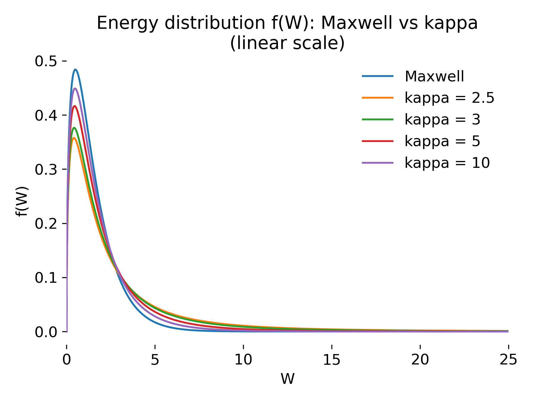
Maxwellian and kappa energy distributions on a linear scale. Energy distributions $f(W)$ for a Maxwellian and several kappa distributions plotted on a linear scale. At low energies, all distributions are dominated by the thermal core and appear similar, illustrating why suprathermal populations can remain hidden in linear representations.

This illustrates an important point: Suprathermal populations can be effectively invisible when focusing only on the bulk of the distribution. In linear representations, the overwhelming majority of particles reside at low energies, masking the presence of rare but energetic particles.

Logarithmic-scale comparison and suprathermal tails

When the same distributions are plotted on a logarithmic scale, the qualitative differences become immediately apparent. The Maxwellian distribution exhibits a straight-line exponential decay in $W$, rapidly dropping below numerical significance at high energies. In contrast, the kappa distributions display extended power-law tails whose slope depends on $\kappa$.

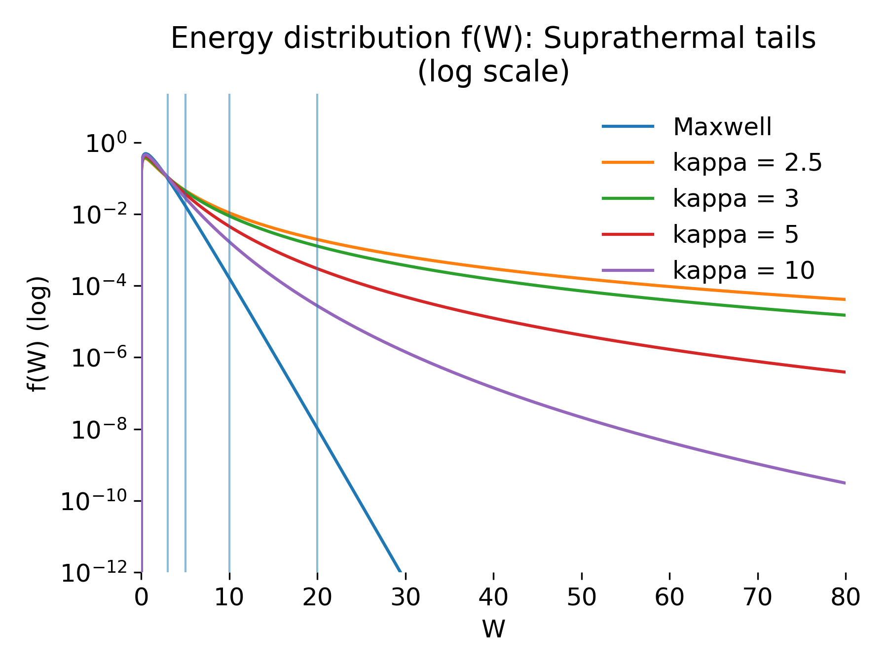
Suprathermal tails revealed on a logarithmic scale. The same energy distributions plotted on a logarithmic scale. The Maxwellian exhibits an exponential decay, while kappa distributions show extended power-law tails whose slope depends on $\kappa$, highlighting the strong enhancement of high-energy particles.

As $\kappa$ decreases, the tail becomes progressively flatter, indicating a substantial enhancement of high-energy particles compared to the Maxwellian case. This behavior is the defining feature of kappa distributions and provides a simple explanation for the ubiquity of suprathermal particles in collisionless plasmas.

Tail fractions above a threshold energy

The tail fraction

\[F(W > W_c) = \int_{W_c}^\infty f(W)\,dW\]

provides a quantitative measure of suprathermal populations. For Maxwellian distributions, this fraction decreases extremely rapidly with increasing $W_c$. Even moderately high thresholds correspond to exponentially small particle fractions.

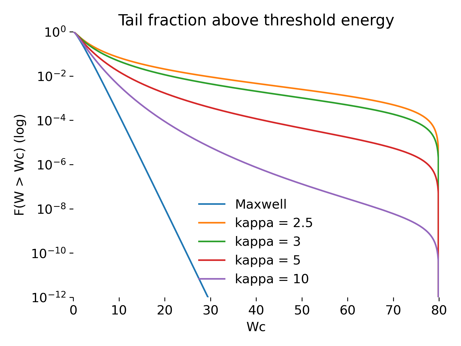
Fraction of particles above a threshold energy. Tail fraction $F(W > W_c)$ as a function of the threshold energy $W_c$ for Maxwellian and kappa distributions. Kappa distributions retain orders of magnitude more particles at high energies compared to the Maxwellian case, demonstrating the physical importance of suprathermal tails in collisionless plasmas.

For kappa distributions, the decay of $F(W > W_c)$ is much slower. At the same threshold energy, the fraction of particles above $W_c$ can exceed the Maxwellian prediction by many orders of magnitude, depending on $\kappa$. This demonstrates that even a small deviation from Maxwellian statistics can dramatically alter the energetic particle content of a plasma.

Physical interpretation with reference to space physics

In space plasmas, suprathermal tails are not an exception but a generic feature. The solar wind, planetary magnetospheres, and heliospheric boundary regions are characterized by long mean free paths and weak collisionality. Under these conditions, particle distributions retain memory of acceleration processes, wave–particle interactions, and boundary effects rather than relaxing to thermal equilibrium.

Kappa distributions provide a compact phenomenological description of these nonthermal populations. The enhanced suprathermal tails play a crucial role in space physics by influencing wave growth rates, collisionless heating, and the efficiency of particle acceleration mechanisms. They also strongly affect moments such as heat flux and higher-order pressure tensors, even when the bulk density and temperature remain well defined.

From this perspective, the comparison presented here illustrates why kinetic models are indispensable in space physics. Fluid models based on Maxwellian closures systematically underestimate the energetic particle content and fail to capture the physics associated with suprathermal populations.

Conclusion

This numerical example demonstrates how Maxwellian and kappa energy distributions differ in their treatment of high-energy particles. While both distributions may appear similar near the thermal core, their tails exhibit fundamentally different behavior that becomes evident on logarithmic scales and through tail-fraction diagnostics.

The results highlight a key lesson of kinetic plasma theory: Rare particles at high energies can dominate important physical processes, even when they represent a small fraction of the total population. Kappa distributions provide a minimal extension of Maxwellian statistics that captures this effect and offers a more realistic description of collisionless space plasmas.

Together with the preceding examples, this comparison reinforces the central role of kinetic descriptions in understanding space plasma dynamics.

Update and code availability: This post and its accompanying Python code were originally drafted in 2020 and archived during the migration of this website to Jekyll and Markdown. In January 2026, I substantially revised and extended the code. The updated and cleaned-up implementation is now available in this new GitHub repositoryꜛ. Please feel free to experiment with it and to share any feedback or suggestions for further improvements.

References and further reading

Wolfgang Baumjohann and Rudolf A. Treumann, Basic Space Plasma Physics, 1997, Imperial College Press, ISBN: 1-86094-079-X
Treumann, R. A., Baumjohann, W., Advanced Space Plasma Physics, 1997, Imperial College Press, ISBN: 978-1-86094-026-2
Donald A. Gurnett, Amitava Bhattacharjee, Introduction to plasma physics with space and laboratory applications, 2005, Cambridge University Press, ISBN: 978-7301245491
Francis F. Chen, Introduction to plasma physics and controlled fusion, 2016, Springer, ISBN: 978-3319223087
R. C. Davidson, Methods in nonlinear plasma theory, 1972, Academic Press, ISBN: 978-0122054501