A spatially developing 2D Kelvin Helmholtz jet with a finite volume projection method

In our previous post we discussed Kelvin-Helmholtz growth in a 2D incompressible shear layer using a vorticity streamfunction formulation on a doubly periodic domain, evolved with a pseudospectral method. Directly building on that, I thought it would be interesting to present an alternative approach that highlights different aspects of both the mathematical formulation and the numerical method.

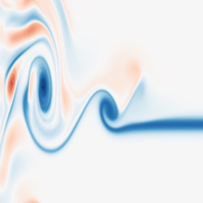
Example of the spatially developing Kelvin-Helmholtz instability in a 2D jet simulated with a finite volume projection method. Shown is the vorticity magnitude $|\omega|$ (color map) overlaid with passive scalar $C$ contours (black lines) at $t=51.2$. The shear layers bounding the jet core have rolled up into coherent Kelvin-Helmholtz billows that advect downstream and interact. The core changes in the numerical code presented in this post are the use of a finite volume discretization on a staggered grid combined with a projection method to evolve the incompressible Navier Stokes equations, as well as the change from a doubly periodic domain to a spatially developing jet with inflow and outflow boundaries.

The same physical mechanism can be explored in a complementary way by switching to a finite volume discretization of the incompressible Navier Stokes equations in primitive variables (velocity and pressure) on a staggered grid. In addition, we will change the domain setup from doubly periodic to a spatially developing jet with inflow and outflow boundaries.

This setup changes the interpretation in an important way. The flow is no longer quasi spatially developing because of periodic wrap around. Instead, perturbations injected near the inlet are convected downstream, grow as they travel, and the observed structures can be associated with genuine downstream development.

Mathematical description

Like before, we consider a 2D incompressible flow of a Newtonian fluid with kinematic viscosity $\nu$ in a rectangular domain of size $L_x\times L_y$. The domain is discretized into $N_x\times N_y$ cells of size $\Delta x=L_x/N_x$ and $\Delta y=L_y/N_y$.

The simulation evolves the incompressible Navier Stokes equations for velocity $\mathbf{u}=(u,v)$ and pressure $p$,

\[\begin{aligned} \partial_t \mathbf{u} + \mathbf{u}\cdot\nabla\mathbf{u} &= -\nabla p + \nu \nabla^2 \mathbf{u}, \\ \nabla\cdot\mathbf{u}&=0, \end{aligned}\]

with constant density absorbed into the pressure definition. In addition, a passive scalar $C(x,y,t)$ is advected by the flow,

\[\partial_t C + \mathbf{u}\cdot\nabla C = \kappa \nabla^2 C,\]

where $\kappa$ is the scalar diffusivity. In the presented runs, $\kappa$ is set to zero or chosen small, so that $C$ primarily visualizes stirring and numerical diffusion.

Projection method and pressure Poisson equation

We will use a standard fractional step projection method in the new numerical set-up. To do so, an intermediate velocity $\mathbf{u}^*$ is computed from advection and diffusion only,

\[\mathbf{u}^* = \mathbf{u}^n + \Delta t\left(-\mathbf{u}\cdot\nabla\mathbf{u} + \nu \nabla^2\mathbf{u}\right),\]

followed by a pressure correction that enforces incompressibility,

\[\mathbf{u}^{n+1} = \mathbf{u}^* - \Delta t \nabla p^{n+1}.\]

Taking the divergence and using $\nabla\cdot\mathbf{u}^{n+1}=0$ yields the Poisson equation

\[\nabla^2 p^{n+1} = \frac{1}{\Delta t}\nabla\cdot\mathbf{u}^*.\]

This is the main conceptual difference to the vorticity streamfunction formulation in the earlier post. There, pressure is eliminated analytically and the elliptic solve is for $\psi$ via $\nabla^2\psi=-\omega$. Here, pressure is solved numerically every step as part of enforcing $\nabla\cdot\mathbf{u}=0$.

Spatially developing jet and boundary conditions

The domain is periodic in $y$ but not periodic in $x$. A jet inflow is imposed at the left boundary by prescribing an inlet profile,

\[u_{\text{in}}(y,t) = U_0\,\mathrm{ramp}(t)\,\exp\!\left(-\left(\frac{y}{w}\right)^2\right),\]

and a small cross stream perturbation is injected via

\[v_{\text{in}}(y,t) = \epsilon U_0\,\mathrm{ramp}(t)\,\sin(2\pi f t)\,\exp\!\left(-\left(\frac{y}{w}\right)^2\right).\]

At the outlet, a convective boundary condition is used for $u$, $v$, and $C$,

\[\begin{aligned} \phi_{\text{out}}^{n+1} &= \phi_{\text{out}}^{n} - \mathrm{CFL}_{\text{out}}\left(\phi_{\text{out}}^{n} - \phi_{\text{in}}^{n}\right),\\ \mathrm{CFL}_{\text{out}} &= U_c\frac{\Delta t}{\Delta x}, \end{aligned}\]

with a convective speed estimate $U_c$. A pressure gauge condition such as $p=0$ at the outlet fixes the null space.

These choices produce a spatially developing flow. Perturbations are introduced at the inlet, then grow and reorganize as they advect downstream.

Relation to Kelvin Helmholtz physics

In this jet configuration, Kelvin Helmholtz type billows are expected on the two shear layers that bound the jet core. A robust diagnostic is therefore the alignment of visible billows in the passive scalar with regions of large vorticity magnitude $|\omega|$, where

\[\omega = \partial_x v - \partial_y u.\]

In shear layer dominated dynamics, coherent billows sit on the vorticity sheets because those sheets are precisely where the velocity gradient and hence the available free energy resides.

Numerical method

In our new setup, we use a finite volume discretization on a staggered grid combined with a projection method to evolve the incompressible Navier Stokes equations. Below are the key aspects of the numerical implementation.

Finite volume discretization on a staggered grid

The code uses a staggered arrangement:

• $u$ on vertical cell faces
• $v$ on horizontal cell faces
• $p$ and $C$ on cell centers

This placement reduces pressure velocity decoupling and makes the discrete divergence and gradient operators naturally compatible in the projection step.

Advection is discretized with a first order upwind choice to maintain robustness for long runs and sharp gradients. Viscous terms are represented by second differences, and the pressure Poisson problem is solved with a mixed strategy: FFT diagonalization in the periodic direction $y$, and a tridiagonal solve in $x$ for each Fourier mode.

Finite volume methods in a nutshell (mathematical and practical view)

Finite volume methods (FVM) are designed to discretize conservation laws in a way that preserves conservation at the discrete level. Their central idea is to evolve cell averages of the conserved quantities by balancing fluxes through the faces of each control volume. This makes FVM particularly well suited for problems where transport and conservation matter and where boundary conditions and non periodic domains are essential.

Why finite volume

A finite volume scheme is built around a statement of integral conservation. For any conserved scalar $q(x,y,t)$ with flux $\mathbf{F}(q)$ and source $S(q)$, the PDE can be written in conservative form as

\[\partial_t q + \nabla\cdot \mathbf{F}(q) = S(q).\]

Integrating over a control volume $V_{ij}$ and using Gauss’ theorem gives

\[\frac{d}{dt}\int_{V_{ij}} q\, dV + \int_{\partial V_{ij}} \mathbf{F}(q)\cdot \mathbf{n}\, dA = \int_{V_{ij}} S(q)\, dV.\]

Finite volume methods discretize this identity directly. Conservation becomes a bookkeeping statement: the time rate of change of the cell content equals the net flux through the faces plus sources.

Cell averages and semidiscrete update

Define the cell average of $q$ over a cell $V_{ij}$ with area $\Delta x\,\Delta y$ as

\[\bar q_{ij}(t) = \frac{1}{\Delta x\,\Delta y}\int_{V_{ij}} q(x,y,t)\, dA.\]

Approximating the surface integrals by numerical fluxes at the cell faces yields the semidiscrete finite volume form

\[\begin{aligned} \frac{d\bar q_{ij}}{dt} =& -\frac{1}{\Delta x}\left(\hat F_{i+\frac12,j}-\hat F_{i-\frac12,j}\right) \\ & -\frac{1}{\Delta y}\left(\hat G_{i,j+\frac12}-\hat G_{i,j-\frac12}\right) +\bar S_{ij}. \end{aligned}\]

Here, $\hat F_{i+\frac12,j}$ and $\hat G_{i,j+\frac12}$ are consistent numerical approximations of the physical flux components through the vertical and horizontal faces. The entire method reduces to specifying

• what quantity is stored as a cell average
• how the face fluxes $\hat F,\hat G$ are computed from neighboring cell values
• how time integration is performed.

Fluxes and upwinding

For pure advection, $q$ satisfies

\[\partial_t q + \nabla\cdot(q\mathbf{u}) = 0,\]

so the physical flux is $\mathbf{F} = q\mathbf{u}$. In finite volume form, the key object is the face flux

\[\begin{aligned} \hat F_{i+\frac12,j} & \approx (q u_x)_{i+\frac12,j}, \\ \hat G_{i,j+\frac12} & \approx (q u_y)_{i,j+\frac12}. \end{aligned}\]

Because information propagates along the flow direction, stable discretizations use upwinding. In the simplest first order upwind form in 1D,

\[\hat F_{i+\frac12} = \begin{cases} u_{i+\frac12}\, q_i, & u_{i+\frac12}\ge 0,\\ u_{i+\frac12}\, q_{i+1}, & u_{i+\frac12}< 0, \end{cases}\]

which is robust but introduces significant numerical diffusion. Higher order variants (MUSCL, TVD limiters, WENO) replace the piecewise constant approximation by reconstructed left and right face values $q_{i+\frac12}^L, q_{i+\frac12}^R$ and then use a flux function

\[\hat F_{i+\frac12} = \mathcal{F}\!\left(q_{i+\frac12}^L, q_{i+\frac12}^R, u_{i+\frac12}\right),\]

with limiters chosen to prevent spurious oscillations near steep gradients.

Diffusion as flux of gradients

Diffusion is naturally handled in the same framework. For

\[\partial_t q = \kappa \nabla^2 q,\]

one writes it in flux form

\[\partial_t q + \nabla\cdot\left(-\kappa \nabla q\right)=0,\]

so the diffusive flux is $\mathbf{F}_{\mathrm{diff}} = -\kappa \nabla q$. In finite volume form, face gradients are approximated by differences between neighboring cell averages, for example

\[\begin{aligned} (\partial_x q)_{i+\frac12,j} &\approx \frac{\bar q_{i+1,j}-\bar q_{i,j}}{\Delta x}, \\ (\partial_y q)_{i,j+\frac12} &\approx \frac{\bar q_{i,j+1}-\bar q_{i,j}}{\Delta y}, \end{aligned}\]

This yields a conservative discrete Laplacian via flux differences.

How this maps to incompressible Navier–Stokes

For incompressible flow, the momentum equation can be written in conservative form as

\[\begin{aligned} \partial_t \mathbf{u} + \nabla\cdot(\mathbf{u}\otimes\mathbf{u}) &= -\nabla p + \nu \nabla^2\mathbf{u}, \\ \nabla\cdot\mathbf{u}&=0. \end{aligned}\]

A finite volume method applies the same control volume idea component wise: the advection term becomes a divergence of momentum fluxes, the viscous term is a divergence of diffusive fluxes, and the pressure gradient acts as a face centered force.

In practice, incompressible FVM is typically coupled to a projection method:

• compute an intermediate velocity from advection and diffusion by evolving the finite volume flux balance
• solve a Poisson equation for pressure to enforce $\nabla\cdot\mathbf{u}=0$
• correct the velocity by subtracting the discrete pressure gradient.

On a staggered grid this is particularly clean because discrete divergence and gradient operators align naturally: $p$ lives at cell centers, while $u$ and $v$ live on faces, exactly where the fluxes are evaluated.

Relevant practical takeaways

In the jet setup of our simulation, finite volume is a natural choice because it handles

• inflow and outflow boundaries without periodic wrap around
• conservative transport of momentum and the passive scalar in a flux based form
• robust long time evolution even when gradients sharpen.

The cost is that the quality of the small scale structures is strongly controlled by the flux scheme (see discussion part). First order upwind is stable but diffusive, which is why early Kelvin–Helmholtz waviness is visually smeared and becomes clear only after energy reaches larger scales.

Pressure solve with FFT in y and tridiagonal solves in x

Because $y$ is periodic, the discrete Laplacian in $y$ is diagonal in Fourier space. For each Fourier mode, the Poisson equation reduces to a 1D Helmholtz type system in $x$ that can be solved efficiently with a Thomas algorithm. This hybrid approach is substantially different from the fully spectral solve on a doubly periodic domain used previously.

Time stepping and stability control

Time stepping is explicit for the advection diffusion part with an adaptive time step based on a CFL condition and a diffusion constraint. This ensures stability even when gradients sharpen and velocities increase locally. As a consequence, the time step is not constant but varies during the simulation.

Numerical implementation in Python

In the following, we walk through the main components of the Python implementation. The full code is available in the GitHub repository linked at the end of this post.

We implement the described finite volume projection method as described above. This means, we need to define shift operators, allocate fields, apply boundary conditions, compute discrete operators (advection, diffusion, divergence, gradients), and solve the pressure Poisson equation.

We begin again by importing necessary libraries and setting some plotting parameters:

import os
import numpy as np
import matplotlib.pyplot as plt
import imageio.v2 as imageio

# remove spines right and top for better aesthetics:
plt.rcParams['axes.spines.right'] = False
plt.rcParams['axes.spines.top'] = False
plt.rcParams['axes.spines.left'] = False
plt.rcParams['axes.spines.bottom'] = False
plt.rcParams.update({'font.size': 12})

The first set of helper functions calculates the shifted versions of arrays needed for finite difference stencils, which is needed for computing derivatives on the staggered grid:

# shift operators:
def shift_x_plus(a):
    return np.concatenate([a[1:, ...], a[-1:, ...]], axis=0)

def shift_x_minus(a):
    return np.concatenate([a[:1, ...], a[:-1, ...]], axis=0)

def shift_y_plus(a):
    return np.roll(a, -1, axis=-1)

def shift_y_minus(a):
    return np.roll(a, 1, axis=-1)

def shift_y_plus_v(a):
    return np.roll(a, -1, axis=1)

def shift_y_minus_v(a):
    return np.roll(a, 1, axis=1)

The next helper function allocates the main fields used in the simulation: velocity components $u$ and $v$, pressure $p$, and passive scalar $C$:

# allocation:
def allocate_fields(Nx, Ny):
    p = np.zeros((Nx, Ny), dtype=float)
    u = np.zeros((Nx + 1, Ny), dtype=float)
    v = np.zeros((Nx, Ny + 1), dtype=float)
    C = np.zeros((Nx, Ny), dtype=float)
    return u, v, p, C

# boundary conditions:
def inlet_profiles(t, params):
    U0 = params["U0"]
    y = params["y_centers"]
    y_faces_v = params["y_faces_v"]
    jet_w = params["jet_w"]
    eps = params["eps"]
    f = params["f"]
    T_ramp = params["T_ramp"]

    # smooth ramp:
    s = np.clip(t / T_ramp, 0.0, 1.0)
    ramp = s * s * (3.0 - 2.0 * s)  # smoothstep

    u_in = (ramp * U0) * np.exp(-(y / jet_w) ** 2)
    v_in = (ramp * eps * U0) * np.sin(2.0 * np.pi * f * t) * np.exp(-(y_faces_v / jet_w) ** 2)
    C_in = np.exp(-(y / jet_w) ** 2)

    return u_in, v_in, C_in, ramp

Additionally, we define a function to apply the boundary conditions at each time step:

def apply_bc(u, v, p, C, t, dt, dx, params):
    """
    y periodic implicit.
    x inlet: Dirichlet for u and v (with ramp)
    x outlet: convective outlet for u, v, C
    pressure gauge at outlet.
    """
    u_in, v_in, C_in, ramp = inlet_profiles(t, params)

    # inlet
    u[0, :] = u_in
    v[0, :] = v_in
    v[0, 0] = v[0, -1]

    C[0, :] = np.maximum(C[0, :], C_in)

    # convective outlet
    # choose a convective speed based on bulk inlet
    Uc = max(params["U0"] * ramp, 1e-6)
    cfl_out = Uc * dt / dx
    cfl_out = min(cfl_out, 0.95)

    # u outlet: u[-1] is boundary face, use u[-2] interior face
    u[-1, :] = u[-1, :] - cfl_out * (u[-1, :] - u[-2, :])

    # v outlet: v[-1] is boundary column of v faces
    v[-1, :] = v[-1, :] - cfl_out * (v[-1, :] - v[-2, :])

    # scalar outlet at centers
    C[-1, :] = C[-1, :] - cfl_out * (C[-1, :] - C[-2, :])

    # pressure gauge
    p[-1, :] = 0.0

Next, we need functions to compute the discrete operators: Laplacians, interpolations, advection, divergence, and pressure gradients:

# operators: laplacians:
def laplacian_center(phi, dx, dy):
    d2x = (shift_x_plus(phi) - 2.0 * phi + shift_x_minus(phi)) / (dx * dx)
    d2y = (shift_y_plus(phi) - 2.0 * phi + shift_y_minus(phi)) / (dy * dy)
    return d2x + d2y

def laplacian_u(u, dx, dy):
    d2x = (shift_x_plus(u) - 2.0 * u + shift_x_minus(u)) / (dx * dx)
    d2y = (shift_y_plus(u) - 2.0 * u + shift_y_minus(u)) / (dy * dy)
    return d2x + d2y

def laplacian_v(v, dx, dy):
    d2x = (shift_x_plus(v) - 2.0 * v + shift_x_minus(v)) / (dx * dx)
    d2y = (shift_y_plus_v(v) - 2.0 * v + shift_y_minus_v(v)) / (dy * dy)
    return d2x + d2y

# interpolations:
def interp_u_to_center(u):
    return 0.5 * (u[:-1, :] + u[1:, :])

def interp_v_to_center(v):
    return 0.5 * (v[:, :-1] + v[:, 1:])

# advection: first order upwind:
def advect_u(u, v, dx, dy):
    Nx1, Ny = u.shape
    v_u = np.zeros((Nx1, Ny), dtype=float)
    v_u[1:-1, :] = 0.25 * (v[:-1, :-1] + v[:-1, 1:] + v[1:, :-1] + v[1:, 1:])
    v_u[0, :] = v_u[1, :]
    v_u[-1, :] = v_u[-2, :]

    dudx_f = (shift_x_plus(u) - u) / dx
    dudx_b = (u - shift_x_minus(u)) / dx
    du_dx = np.where(u >= 0.0, dudx_b, dudx_f)

    dudy_f = (shift_y_plus(u) - u) / dy
    dudy_b = (u - shift_y_minus(u)) / dy
    du_dy = np.where(v_u >= 0.0, dudy_b, dudy_f)

    return u * du_dx + v_u * du_dy


def advect_v(u, v, dx, dy):
    Nx, Ny1 = v.shape
    u_v = np.zeros((Nx, Ny1), dtype=float)
    u_v[:, 1:-1] = 0.25 * (u[:-1, :-1] + u[1:, :-1] + u[:-1, 1:] + u[1:, 1:])
    u_v[:, 0] = u_v[:, 1]
    u_v[:, -1] = u_v[:, -2]

    dvdx_f = (shift_x_plus(v) - v) / dx
    dvdx_b = (v - shift_x_minus(v)) / dx
    dv_dx = np.where(u_v >= 0.0, dvdx_b, dvdx_f)

    dvdy_f = (shift_y_plus_v(v) - v) / dy
    dvdy_b = (v - shift_y_minus_v(v)) / dy
    dv_dy = np.where(v >= 0.0, dvdy_b, dvdy_f)

    return u_v * dv_dx + v * dv_dy

We also need functions for computing the divergence of the intermediate velocity and the pressure gradients needed for the projection step:

# divergence and pressure gradients:
def divergence(u, v, dx, dy):
    return (u[1:, :] - u[:-1, :]) / dx + (v[:, 1:] - v[:, :-1]) / dy

def grad_p_to_u(p, dx):
    gp = np.zeros((p.shape[0] + 1, p.shape[1]), dtype=float)
    gp[1:-1, :] = (p[1:, :] - p[:-1, :]) / dx
    gp[0, :] = gp[1, :]
    gp[-1, :] = gp[-2, :]
    return gp

def grad_p_to_v(p, dy):
    gp = np.zeros((p.shape[0], p.shape[1] + 1), dtype=float)
    gp[:, 1:-1] = (p[:, 1:] - p[:, :-1]) / dy
    gp[:, 0] = gp[:, -2]
    gp[:, -1] = gp[:, 1]
    return gp

We still need to implement the Poisson solver for pressure using FFT in $y$ and tridiagonal solves in $x$:

# Poisson solver: SOR
def solve_poisson_fft_y(p, rhs, dx, dy):
    """
    Solve ∇² p = rhs on cell centers with periodic y via FFT.

    Discretization
    * y is periodic, so FFT diagonalizes the y Laplacian
    * for each ky mode we solve a 1D Helmholtz system in x:
        (Dxx - k_y^2) p_hat = rhs_hat
      with
        Neumann at inlet (x=0): p[0] = p[1]
        Dirichlet at outlet (x=Lx): p[Nx-1] = 0

    Returns updated p (real).
    """
    Nx, Ny = rhs.shape

    # FFT in y:
    rhs_hat = np.fft.fft(rhs, axis=1)

    # wavenumbers in y for discrete Laplacian eigenvalues
    # for second difference operator in y:
    # λ_y(ky) = (2 cos(ky dy) - 2) / dy^2 = -4 sin^2(ky dy / 2) / dy^2
    ky = 2.0 * np.pi * np.fft.fftfreq(Ny, d=dy)
    lam_y = -4.0 * (np.sin(0.5 * ky * dy) ** 2) / (dy * dy)  # shape (Ny,)

    # preallocate solution in Fourier space:
    p_hat = np.zeros_like(rhs_hat, dtype=np.complex128)

    # tridiagonal coefficients for x operator:
    ax = 1.0 / (dx * dx)   # sub diagonal
    cx = 1.0 / (dx * dx)   # super diagonal
    # main diagonal depends on mode: bx = -2/dx^2 + lam_y[m]
    # because (Dxx + Dyy) p = rhs, and Dyy eigenvalue is lam_y

    # Thomas solver for each mode in y:
    for m in range(Ny):
        b0 = (-2.0 / (dx * dx) + lam_y[m])  # main diagonal value for this mode

        # build diagonals
        a = ax * np.ones(Nx - 1, dtype=np.complex128)
        b = b0 * np.ones(Nx, dtype=np.complex128)
        c = cx * np.ones(Nx - 1, dtype=np.complex128)
        d = rhs_hat[:, m].astype(np.complex128)

        # apply BCs:
        # Neumann at i=0: p0 - p1 = 0
        b[0] = 1.0
        c[0] = -1.0
        d[0] = 0.0

        # Dirichlet at i=Nx-1: p = 0
        a[-1] = 0.0
        b[-1] = 1.0
        d[-1] = 0.0

        # forward elimination:
        for i in range(1, Nx):
            w = a[i - 1] / b[i - 1]
            b[i] = b[i] - w * c[i - 1]
            d[i] = d[i] - w * d[i - 1]

        # back substitution:
        x = np.zeros(Nx, dtype=np.complex128)
        x[-1] = d[-1] / b[-1]
        for i in range(Nx - 2, -1, -1):
            x[i] = (d[i] - c[i] * x[i + 1]) / b[i]

        p_hat[:, m] = x

    # inverse FFT back to real space:
    p_new = np.fft.ifft(p_hat, axis=1).real

    # Gauge fix at outlet:
    p_new[-1, :] = 0.0
    # inlet Neumann consistency:
    p_new[0, :] = p_new[1, :]

    return p_new

Also needed is the advection of the passive scalar:

# passive scalar:
def advect_scalar(C, u, v, dx, dy):
    uc = interp_u_to_center(u)
    vc = interp_v_to_center(v)

    Cx_f = (shift_x_plus(C) - C) / dx
    Cx_b = (C - shift_x_minus(C)) / dx
    dC_dx = np.where(uc >= 0.0, Cx_b, Cx_f)

    Cy_f = (shift_y_plus(C) - C) / dy
    Cy_b = (C - shift_y_minus(C)) / dy
    dC_dy = np.where(vc >= 0.0, Cy_b, Cy_f)

    return uc * dC_dx + vc * dC_dy

# diagnostics and plotting:
def compute_vorticity(u, v, dx, dy):
    v_mid = 0.5 * (v[:, :-1] + v[:, 1:])
    dv_dx = (shift_x_plus(v_mid) - shift_x_minus(v_mid)) / (2.0 * dx)
    u_mid = 0.5 * (u[:-1, :] + u[1:, :])
    du_dy = (shift_y_plus(u_mid) - shift_y_minus(u_mid)) / (2.0 * dy)
    return dv_dx - du_dy

The next set of functions handle the visualization of the simulation results, including saving frames and rendering images:

def save_frame(frame_path, x_centers, y_centers, field, title, vmin=None, vmax=None,
               ylim=None):
    """ 
    Save a field plot to file.
    
    Parameters
    ----------
    field : (Nx, Ny) array, field on cell centers
    title : str, plot title
    frame_path : str, path to save the plot
    vmin, vmax : float, optional, color limits
    ylim : tuple, optional, y-axis limits
    """
    plt.figure(figsize=(10, 5), dpi=140)
    extent = [x_centers[0], x_centers[-1], y_centers[0], y_centers[-1]]
    plt.imshow(field.T, origin="lower", extent=extent, aspect="auto", vmin=vmin, vmax=vmax,
               cmap="RdBu_r")
    plt.xlabel("x")
    plt.ylabel("y")
    if ylim is not None:
        plt.ylim(ylim)
    plt.title(title)
    plt.tight_layout()
    plt.savefig(frame_path)
    plt.close()

def save_overlay_frame(frame_path, x_centers, y_centers, omega, C,
                       title,
                       omega_percentile=99.0,
                       C_levels=10,
                       ylim=None):
    """
    Plot vorticity ω as background and overlay passive scalar C as contour lines.
    This makes it easy to see whether the billows in C sit on the shear layers
    where |ω| is large.

    Parameters
    ----------
    omega : (Nx, Ny) array, vorticity on cell centers
    C     : (Nx, Ny) array, passive scalar on cell centers
    """
    plt.figure(figsize=(10, 5), dpi=140)

    extent = [x_centers[0], x_centers[-1], y_centers[0], y_centers[-1]]

    # robust symmetric color limits for ω
    clim = np.percentile(np.abs(omega), omega_percentile)
    clim = max(clim, 1e-12)

    # background ω
    plt.imshow(omega.T, origin="lower", extent=extent, aspect="auto",
               vmin=-clim, vmax=clim, cmap="RdBu_r")

    # overlay C contours (use original C, not gamma-corrected)
    # choose contour levels between min and max, but avoid a degenerate range
    cmin = float(np.min(C))
    cmax = float(np.max(C))
    if cmax - cmin < 1e-12:
        levels = np.linspace(0.0, 1.0, C_levels)
    else:
        levels = np.linspace(cmin + 0.05*(cmax - cmin), cmax - 0.05*(cmax - cmin), C_levels)

    plt.contour(x_centers, y_centers, C.T, levels=levels, linewidths=1.0)

    plt.xlabel("x")
    plt.ylabel("y")
    if ylim is not None:
        plt.ylim(ylim)
    plt.title(title)
    plt.tight_layout()
    plt.savefig(frame_path)
    plt.close()

def fig_to_rgb_array(fig):
    """
    Convert a Matplotlib figure to an RGB uint8 array (H, W, 3).
    Works with the Agg backend that is default in non-interactive scripts.
    """
    fig.canvas.draw()
    rgba = np.asarray(fig.canvas.buffer_rgba(), dtype=np.uint8)  # (H, W, 4)
    rgb = rgba[..., :3].copy()  # drop alpha
    return rgb

def render_frame_rgb(x_centers, y_centers, field, title, vmin=None, vmax=None,
                     ylim=None, cmap="RdBu_r"):
    """ 
    Render a field plot to an RGB uint8 array (H, W, 3).
    
    Parameters
    ----------
    field : (Nx, Ny) array, field on cell centers
    title : str, plot title
    vmin, vmax : float, optional, color limits
    ylim : tuple, optional, y-axis limits
    cmap : str, optional, colormap
    """
    fig = plt.figure(figsize=(10, 5), dpi=140)
    extent = [x_centers[0], x_centers[-1], y_centers[0], y_centers[-1]]
    plt.imshow(field.T, origin="lower", extent=extent, aspect="auto",
               vmin=vmin, vmax=vmax, cmap=cmap)
    plt.xlabel("x")
    plt.ylabel("y")
    if ylim is not None:
        plt.ylim(ylim)
    plt.title(title)
    plt.tight_layout()

    frame = fig_to_rgb_array(fig)
    plt.close(fig)
    return frame

def render_overlay_rgb(x_centers, y_centers, omega, C, title,
                       omega_percentile=99.0, C_levels=10, ylim=None):
    """ 
    Render vorticity ω as background and overlay passive scalar C as contour lines
    to an RGB uint8 array (H, W, 3).
    
    Parameters
    ----------
    omega : (Nx, Ny) array, vorticity on cell centers
    C     : (Nx, Ny) array, passive scalar on cell centers
    title : str, plot title
    omega_percentile : float, percentile for robust color limits of ω
    C_levels : int, number of contour levels for C
    ylim : tuple, optional, y-axis limits
    """
    fig = plt.figure(figsize=(10, 5), dpi=140)
    extent = [x_centers[0], x_centers[-1], y_centers[0], y_centers[-1]]

    clim = np.percentile(np.abs(omega), omega_percentile)
    clim = max(clim, 1e-12)

    plt.imshow(omega.T, origin="lower", extent=extent, aspect="auto",
               vmin=-clim, vmax=clim, cmap="RdBu_r")

    cmin = float(np.min(C))
    cmax = float(np.max(C))
    if cmax - cmin < 1e-12:
        levels = np.linspace(0.0, 1.0, C_levels)
    else:
        levels = np.linspace(cmin + 0.05*(cmax - cmin), cmax - 0.05*(cmax - cmin), C_levels)

    plt.contour(x_centers, y_centers, C.T, levels=levels, linewidths=1.0)

    plt.xlabel("x")
    plt.ylabel("y")
    if ylim is not None:
        plt.ylim(ylim)
    plt.title(title)
    plt.tight_layout()

    frame = fig_to_rgb_array(fig)
    plt.close(fig)
    return frame

Now that all helper functions are defined, we can set up the simulation parameters. We begin by defining output directories for saving frames and GIFs:

# output settings:
out_dir = "kh_fv_output"
frames_dir = os.path.join(out_dir, "frames")
frames_dir_C = os.path.join(out_dir, "frames_C")
frames_dir_overlay = os.path.join(out_dir, "frames_overlay")
os.makedirs(frames_dir, exist_ok=True)
os.makedirs(frames_dir_C, exist_ok=True)
os.makedirs(frames_dir_overlay, exist_ok=True)
gif_path = os.path.join(out_dir, "kh_finite_volume_omega.gif")
gif_path_C = os.path.join(out_dir, "kh_finite_volume_C.gif")
gif_path_overlay = os.path.join(out_dir, "kh_finite_volume_overlay.gif")

Next and most importantly, we define the physical and numerical parameters for the simulation. We will implement a spatially developing jet with a Kelvin Helmholtz instability using a simulation box of size $L_x \times L_y$ (here: 300.0 \times 70.0) discretized on a grid of $N_x \times N_y$ points (here: 720 \times 320). The jet has a maximum velocity $U_0=1.5$ and half-width $jet_w=3.0$. The Reynolds number $Re=300$ controls the viscosity $\nu$ (which depends on $U_0$ and $jet_w$). The passive scalar diffusivity $\kappa$ is set to zero or a small fraction of $\nu$. The inlet perturbation amplitude $\epsilon=0.06$ and frequency $f=0.06$ are also specified. The simulation runs until time $t_{\text{end}}$ (here: 800), saving frames at regular intervals:

Lx = 300.0 # domain size in x
Ly = 70.0  # domain size in y
Nx = 360*2   # grid points in x; start with 360; the higher the better but also computationally more expensive
Ny = 160*2   # grid points in y; start with 160; the higher the better but also computationally more expensive

dx = Lx / Nx # grid spacing in x
dy = Ly / Ny # grid spacing in y

x_centers = (np.arange(Nx) + 0.5) * dx
y_centers = (np.arange(Ny) + 0.5) * dy - 0.5 * Ly
y_faces_v = np.arange(Ny + 1) * dy - 0.5 * Ly

U0 = 1.5    # jet max velocity; start with 1.0
jet_w = 3.0  # jet half width
Re = 300.0  # start more viscous for stability, later increase again
nu = U0 * jet_w / Re  # kinematic viscosity
#kappa = 0.25 * nu  # passive scalar diffusivity
kappa = 0.00 * nu

eps = 0.06
f = 0.06
T_ramp = 8.0

CFL = 0.20
dt_max = 0.04

t_end = 800.0
target_frames = 220
frame_dt = t_end / target_frames

Before starting the time-stepping loop, we allocate the fields and set the initial conditions. The velocity fields $u$ and $v$ are initialized to zero, and the passive scalar $C$ is also initialized to zero:

u, v, p, C = allocate_fields(Nx, Ny)

params = {
    "U0": U0,
    "jet_w": jet_w,
    "eps": eps,
    "f": f,
    "T_ramp": T_ramp,
    "y_centers": y_centers,
    "y_faces_v": y_faces_v,
}

# mild initial condition, almost rest, with a weak jet shape
u[:, :] = 0.0
v[:, :] = 0.0
C[:, :] = 0.0

Now, we can finally implement the main time-stepping loop. In each iteration, we compute an adaptive time step based on the CFL condition and diffusion constraint, apply boundary conditions, compute advection and diffusion terms, perform the projection step to enforce incompressibility, and update the passive scalar. We also save frames at specified intervals for later visualization:

t = 0.0
next_frame_t = 0.0
frames = []
frames_C = []
frames_overlay = []
frame_idx = 0

while t < t_end:
    # adaptive dt based on current max velocity:
    umax = np.max(np.abs(u))
    vmax = np.max(np.abs(v))
    u_char = max(umax, vmax, 1e-6)
    dt_adv = CFL * min(dx, dy) / u_char
    dt_diff = 0.20 * min(dx, dy) ** 2 / max(nu, 1e-12)
    dt = min(dt_adv, dt_diff, dt_max, frame_dt)

    apply_bc(u, v, p, C, t=t, dt=dt, dx=dx, params=params)

    adv_u = advect_u(u, v, dx, dy)
    adv_v = advect_v(u, v, dx, dy)

    diff_u = nu * laplacian_u(u, dx, dy)
    diff_v = nu * laplacian_v(v, dx, dy)

    u_star = u + dt * (-adv_u + diff_u)
    v_star = v + dt * (-adv_v + diff_v)

    apply_bc(u_star, v_star, p, C, t=t, dt=dt, dx=dx, params=params)

    div_star = divergence(u_star, v_star, dx, dy)
    rhs = div_star / dt
    rhs -= np.mean(rhs)

    # diagnostic clamp to avoid catastrophic SOR RHS in case of reflections:
    rhs_clip = 1e3
    rhs = np.clip(rhs, -rhs_clip, rhs_clip)
    
    # secure against NaNs/Infs:
    div_star = divergence(u_star, v_star, dx, dy)
    rhs = div_star / dt
    rhs -= np.mean(rhs)
    rhs = np.nan_to_num(rhs, nan=0.0, posinf=0.0, neginf=0.0)

    # solve for pressure:
    p = solve_poisson_fft_y(p, rhs, dx, dy)

    u = u_star - dt * grad_p_to_u(p, dx)
    v = v_star - dt * grad_p_to_v(p, dy)

    apply_bc(u, v, p, C, t=t, dt=dt, dx=dx, params=params)

    adv_C = advect_scalar(C, u, v, dx, dy)
    diff_C = kappa * laplacian_center(C, dx, dy)
    C = C + dt * (-adv_C + diff_C)
    C = np.clip(C, 0.0, 1.0)
    apply_bc(u, v, p, C, t=t, dt=dt, dx=dx, params=params)

    if not (np.isfinite(u).all() and np.isfinite(v).all() and np.isfinite(p).all()):
        raise FloatingPointError("Non finite values. Further reduce CFL/dt_max or increase viscosity.")

    if t >= next_frame_t or t + dt >= t_end:
        omega_field = compute_vorticity(u, v, dx, dy)
        
        
        # omega plot:
        field_to_plot = omega_field
        title = f"2D KH, t = {t:7.2f}, Re = {Re:g}, dt = {dt:.3e} (omega field)"
        frame_path = os.path.join(frames_dir, f"frame_{frame_idx:05d}.png")
        clim = np.percentile(np.abs(field_to_plot), 99.0)
        clim = max(clim, 1e-6)
        save_frame(frame_path, x_centers, y_centers, field_to_plot, title, vmin=-clim, vmax=clim)
        omega_rgb = render_frame_rgb(x_centers, y_centers, omega_field, title,
                             vmin=-clim, vmax=clim, cmap="RdBu_r")
        frames.append(omega_rgb)
        #frames.append(imageio.imread(frame_path))
        print(f"Saved {frame_path}")
        
        
        # plot C:
        field_to_plot = C
        # Gamma correction of c/field_to_pot for better visibility:
        field_to_plot_gamma = field_to_plot ** 0.6
        title = f"2D KH, t = {t:7.2f}, Re = {Re:g}, dt = {dt:.3e} (Passive Scalar C)"
        frame_path = os.path.join(frames_dir_C, f"frame_{frame_idx:05d}.png")
        save_frame(frame_path, x_centers, y_centers, field_to_plot_gamma, title, vmin=0.0, vmax=1.0)
        # render C to RAM:
        C_rgb = render_frame_rgb(x_centers, y_centers, field_to_plot_gamma, title,
                                vmin=0.0, vmax=1.0, cmap="Reds")
        frames_C.append(C_rgb)
        #frames_C.append(imageio.imread(frame_path))
        print(f"Saved {frame_path}")
        
        
        # overlay plot ω background + C contours:
        title = f"2D KH overlay, t = {t:7.2f}, Re = {Re:g}, dt = {dt:.3e} (ω + C contours)"
        frame_path = os.path.join(frames_dir_overlay, f"frame_{frame_idx:05d}.png")
        save_overlay_frame(frame_path, x_centers, y_centers, omega_field, C, title, omega_percentile=99.0, C_levels=12)
        # overlay: render to RAM
        overlay_rgb = render_overlay_rgb(x_centers, y_centers,
                                        omega=omega_field, C=C, title=title,
                                        omega_percentile=99.0, C_levels=12)
        frames_overlay.append(overlay_rgb)
        #frames_overlay.append(imageio.imread(frame_path))
        print(f"Saved {frame_path}")
        
        frame_idx += 1
        next_frame_t += frame_dt

    t += dt

When the simulation is complete, we save the collected frames as GIF animations for visualization:

imageio.mimsave(gif_path, frames, duration=0.06, plugin="pillow", palettesize=256, subrectangles=False)
imageio.mimsave(gif_path_C, frames_C, duration=0.06, plugin="pillow", palettesize=256, subrectangles=False)
imageio.mimsave(gif_path_overlay, frames_overlay, duration=0.06, plugin="pillow", palettesize=256, subrectangles=False)
print("All GIFs saved.")

Simulation results and discussion

The three animations below show the same simulation from complementary viewpoints. The passive scalar $C$ visualizes material transport and mixing, the vorticity field $\omega$ highlights where shear and rotation concentrate, and the overlay directly tests whether the visible scalar billows sit on the shear layers where $|\omega|$ is large:

Resulting GIFs: Time evolution of a 2D incompressible starting jet. Top: passive scalar $C$ injected at the inlet. Middle: vorticity $\omega = \partial_x v - \partial_y u$ computed from the staggered velocity field. Bottom: overlay of $\omega$ (background) with $C$ contour lines. The overlay is the key diagnostic for Kelvin–Helmholtz type dynamics because KH billows must coincide with the shear layers where $|\omega|$ is maximal.

What the animations show, in brief

At first glance, we see a jet entering from the left, with a compact “head” region followed by a trailing jet core. The jet edges display growing waviness that eventually rolls up into vortical structures. This is qualitatively the expected Kelvin–Helmholtz instability behavior for a spatially developing shear layer.

So, what is going on physically? The leading “head” should not be confused with a shock front, e.g., a “bow shock”-like structure. This does not fit the physics of this model. The code evolves incompressible Navier–Stokes without compressibility, without an energy equation, and without an equation of state. There are no acoustic characteristics, hence no genuine shock fronts. Any feature that visually resembles a “front” must be one of the following:

• a very steep gradient region of the passive scalar $C$ (contours crowd together)
• a region of strongly concentrated vorticity in a shear layer
• a startup transient of the jet injection that generates a dominant head vortex
• numerical effects of the advective discretization (first order upwind is robust but strongly diffusive and shapes fronts differently from higher order schemes)

The simulation is dominated early by a classic starting jet transient. The inlet profile is ramped in time (via T_ramp) while the entire domain is initialized with $u=v=C=0$. As the jet accelerates into a quiescent ambient fluid, a strong shear zone forms at the advancing jet front. This rapidly produces a large scale coherent vortical structure at the jet tip, the “head vortex”. In 3D, the analog would be a starting vortex ring; in 2D it appears as a vortex pair or a large roll up structure that leads the jet. This head vortex is not a shock. It is coherent vorticity that strongly organizes the downstream flow and delays the moment when the trailing shear layers display the textbook Kelvin–Helmholtz billows.

Kelvin–Helmholtz dynamics do occur along the jet edges, but with an important precision: In a spatially developing shear layer, KH growth is convective. Perturbations amplify while being advected downstream. It is therefore plausible that clean roll up becomes visually obvious only beyond some distance $x$ (here: somewhere between $x=100-150$). Where that distance sits depends on the effective shear layer thickness, Reynolds number, inlet perturbation amplitude and frequency, and the effective numerical viscosity introduced by the scheme. In our code, strict first order upwind advection introduces strong numerical dissipation, which smears small scales, so early KH waviness can remain faint until larger structures emerge.

The clean physical test for KH is also visible in the overlay. KH billows must sit on the shear layers. Quantitatively, the billows in $C$ should track the locations where $|\omega|$ is largest along the jet edges, because for a jet dominated by streamwise velocity $u(y)$ one expects approximately

\[\omega \approx -\frac{\partial u}{\partial y}.\]

In the overlay frames, the densest $C$ contours align with regions of strong $|\omega|$ along the upper and lower jet boundaries, and later wrap around vortical cores. That is consistent with KH behavior superimposed on a strong starting jet head vortex.

Snapshot sequence

The following snapshots isolate key stages. Each block shows (top to bottom) $C$, $\omega$, and the overlay $\omega$ plus $C$ contours at the same time.

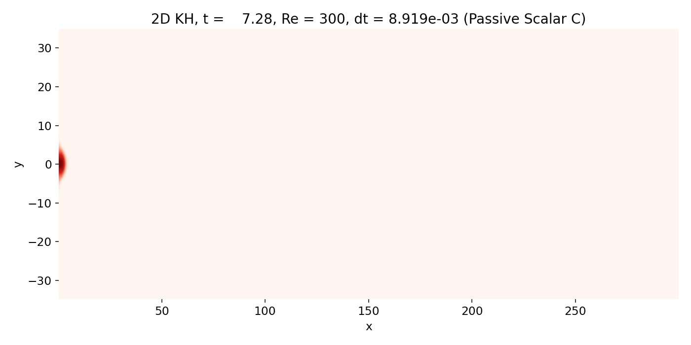
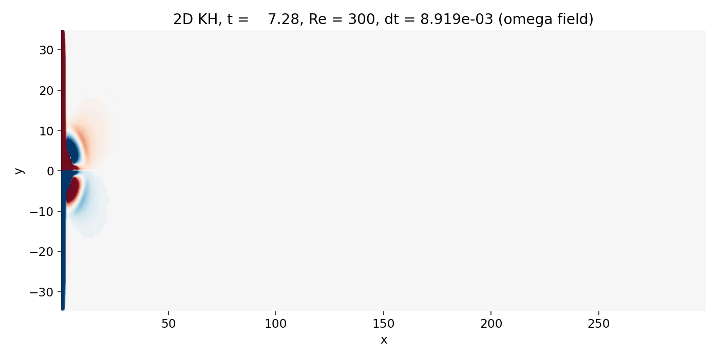
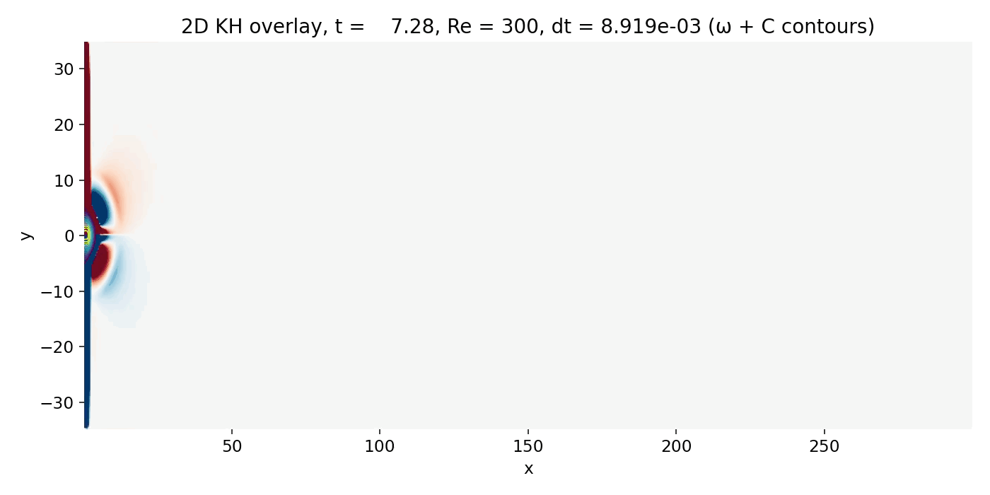
Initializing time: Starting jet phase

At early times, essentially everything is a startup transient. Because the inlet velocity is being ramped from rest, the problem is not a statistically steady spatially developing mixing layer but a starting jet that accelerates into a quiescent ambient. The scalar $C$ shows a bulb like “head” at the leading edge (see earlier discussion), with sharp gradients at its boundary. Those sharp gradients can look “front like”, but they are purely advective steepening plus numerical diffusion, not compressible shock physics.

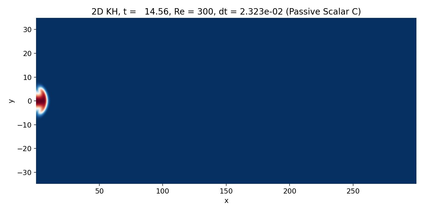
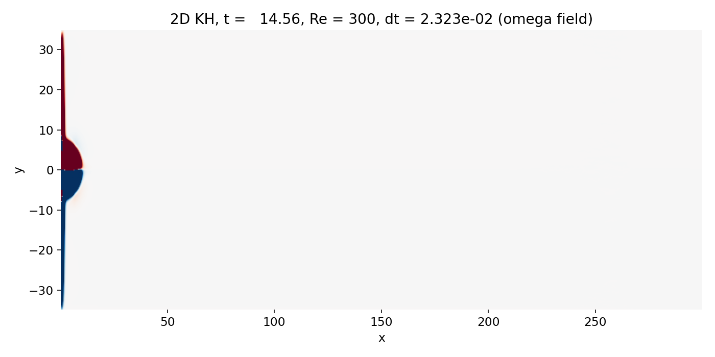
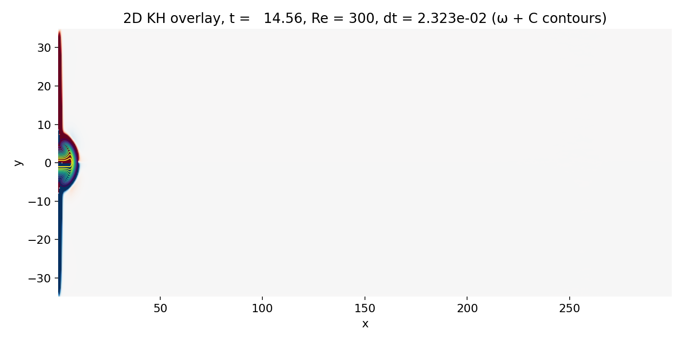
Early starting jet phase (frame 00004, $t \approx 14.6$). The injected scalar forms a compact head and a narrow trailing jet core. Vorticity is concentrated on the upper and lower shear layers and already begins to organize the flow near the jet front.

The vorticity field already shows the key structures: Two bands of opposite sign along the jet edges, where the shear is maximal. The overlay confirms that the tightest $C$ contours sit on these vorticity bands. This is the correct physical reading: the visible interface is a shear layer, and the relevant instability mechanism is shear driven vorticity dynamics.

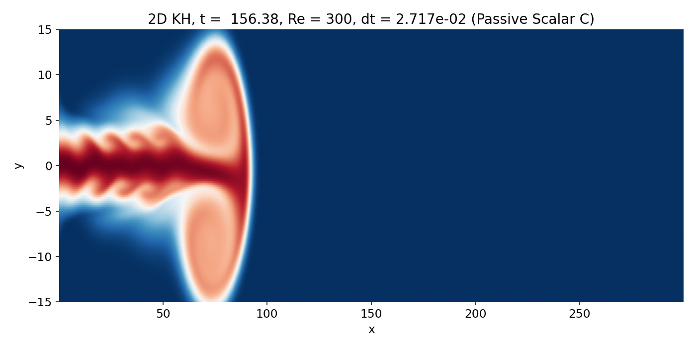
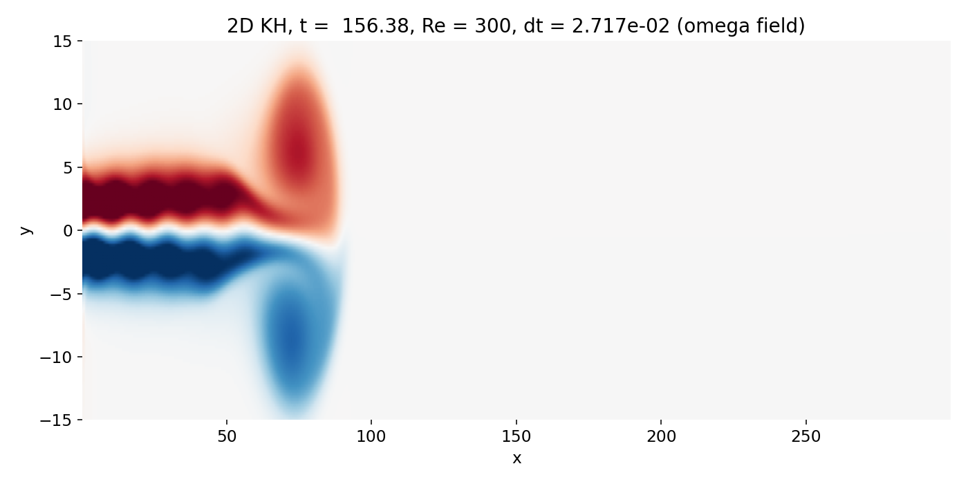
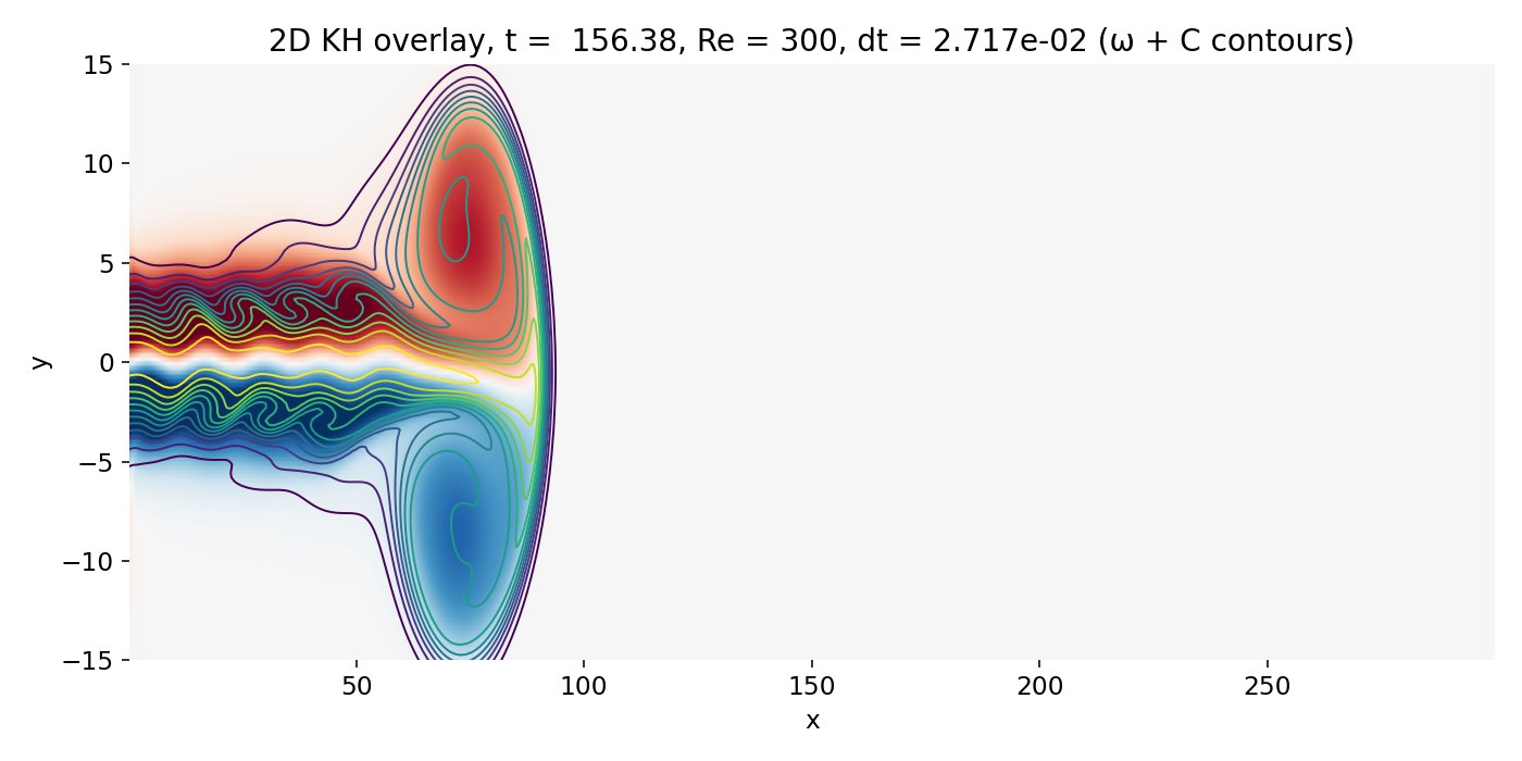
Early time: Jet head vortex formation

As the jet continues to accelerate, the head vortex forms and strengthens. The scalar head has grown into a large coherent lobe and the vorticity field shows a paired, large scale structure at the front, with opposite signs in the upper and lower halves. This is the 2D analog of the starting vortex ring concept: The jet front generates a strong shear layer against the ambient, which rapidly rolls up into a dominant vortical complex.

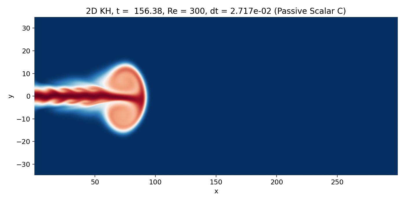
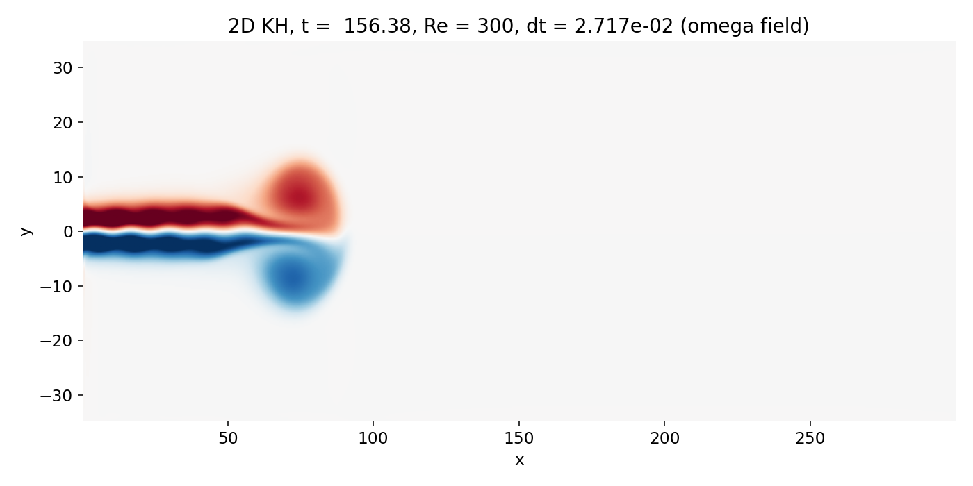
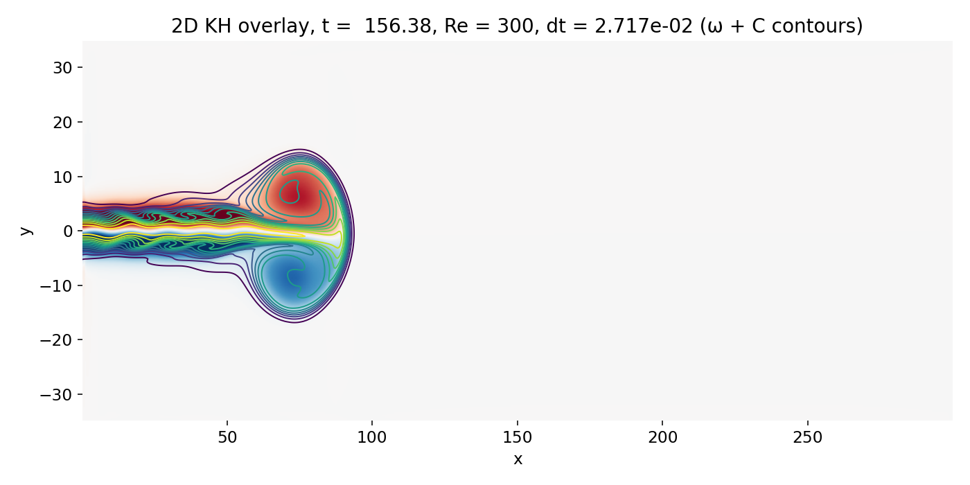
Fully developed head vortex pair at the jet tip (frame 00043, $t \approx 156.4$). The scalar head becomes a large coherent lobe, and the vorticity field shows a dominant large scale roll up structure that controls the near wake.

This structure is not “Kelvin–Helmholtz billows of a parallel mixing layer” in the narrow textbook sense. It is a jet head phenomenon that exists even without a sustained upstream mixing layer instability. It matters because it imposes a large scale velocity field and induces global deflection and recirculation, which the trailing shear layers inherit. Any KH growth behind it occurs in a background flow that is already strongly distorted.

The overlay remains the most informative. The $C$ contours wrap around the head vortex, and the densest contour packing coincides with strong $|\omega|$ on the jet boundary, confirming that the scalar structures are shear layer features shaped by vorticity dynamics.

Intermediate time: Transition to downstream shear layer dynamics

As time progresses, the head vortex moves downstream and the trailing shear layers begin to show waviness. The jet centerline is visibly deflected, and the scalar distribution shows a stretched head with a trailing column. The vorticity field reveals that the strongest shear is still concentrated in the upper and lower boundary layers of the jet. These are the sites where KH growth can occur.

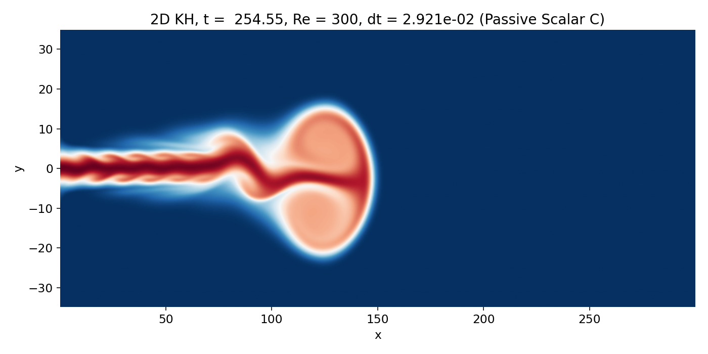
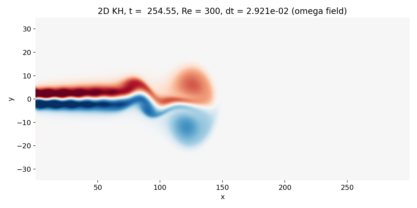
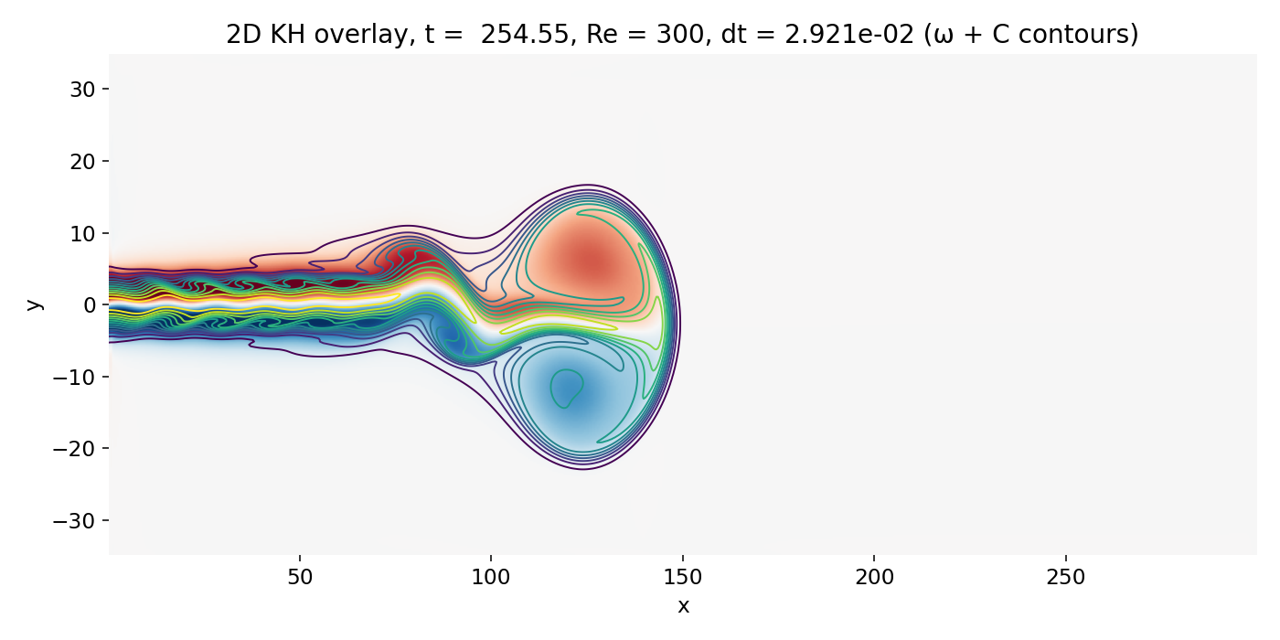
Transition from head dominated dynamics to downstream shear layer dynamics (frame 00070, $t \approx 254.6$). The head vortex advects and deforms the jet, while the trailing shear layers begin to show coherent waviness that can grow convectively.

Two processes are entangled here.

First, convective KH growth along the shear layers: perturbations introduced at the inlet, especially through the imposed transverse inlet velocity modulation $v_{\mathrm{in}}(t)$, are carried downstream and can amplify while traveling.

Second, wake dynamics in the head vortex flow: the large scale induced velocities and curvature generated by the head vortex change the effective shear layer geometry. This can make trailing structures look like “instability onset” at some $x$, when in fact the perturbations have been present earlier but were either too small to see or were smeared by numerical diffusion.

In our code, first order upwind advection is a strong smoothing operator. It suppresses small scale roll up and makes early KH waviness appear softer than it would under a higher order flux reconstruction. This is why early edge billows look comparatively unspecific and become visually compelling only once they reach large amplitude and scale.

Late time: Nonlinear coherent structure emergence downstream

At later times, large scale coherent vortices appear downstream of the jet head. In the scalar field, large lobes appear and the jet boundary becomes strongly deformed. In vorticity, broad regions of opposite sign form and separate, indicating that the shear layers have rolled up into large scale vortical cells. The overlay shows the decisive correlation: $C$ contours fold and wrap around these vorticity concentrations.

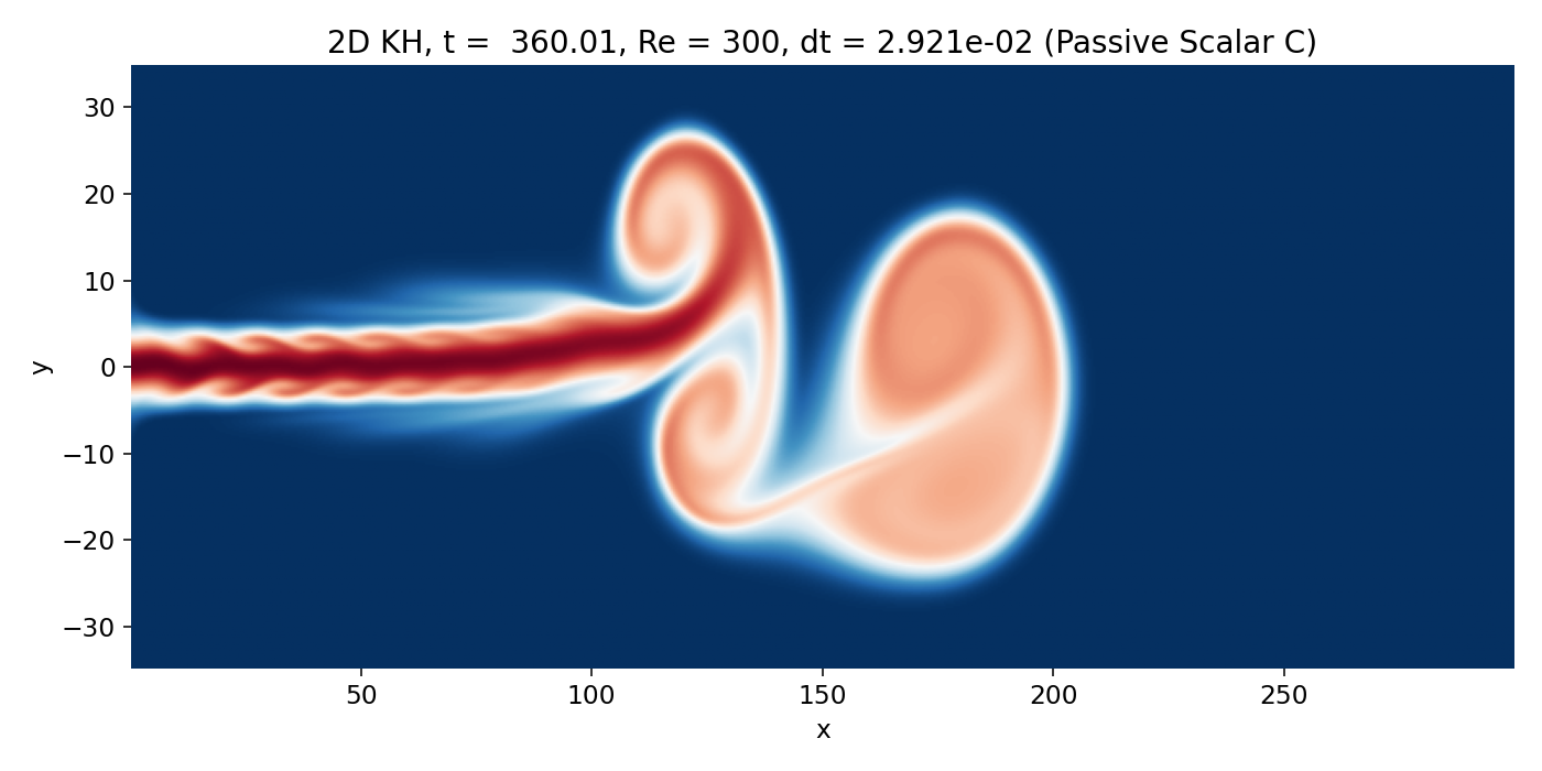
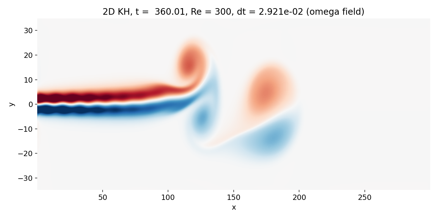
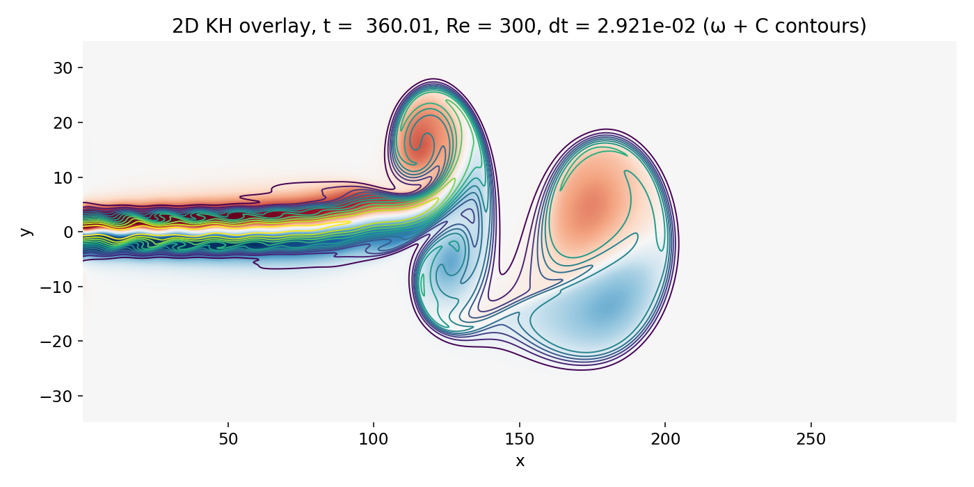
Emergence of large scale coherent vortices downstream of the jet head (frame 00099, $t \approx 360.0$). Scalar lobes form as the shear layers roll up and the contours wrap around regions of strong vorticity.

This is the regime where it is appropriate to say that the flow exhibits Kelvin–Helmholtz type roll up along the jet shear layers. The key point is that the instability is not “starting at $x \approx 150$” in a strict sense. What becomes obvious around that region is the nonlinear visibility threshold of coherent structures that survived numerical dissipation and grew to large amplitude. Upstream of that, there can be genuine KH growth, but its early manifestations are faint and heavily shaped by the head vortex background and by the dissipative advection scheme.

The large structures downstream can arise from a mixture of mechanisms:

• KH roll up along the upper and lower shear layers
• pairing and merger of vortices into fewer, larger structures, which is particularly pronounced in 2D because inverse energy transfer favors growth of large scales
• advection and deformation imposed by the head vortex induced velocity field, which bends and stretches the shear layers and biases where coherent structures appear

The images show all three qualitatively, but KH remains the central generator of roll up along the jet boundaries.

Further progression: Strongly nonlinear regime with dominant vortices

At very late times, the flow is dominated by a few large scale coherent vortices downstream (beyond $x \gtrsim 150$) of the jet head. The upstream jet core is still relatively straight, while downstream the jet shear layers undergo large scale deformation into a small number of dominant coherent structures. In the vorticity plot, the structures appear smooth and extended rather than filled with fine filaments. That smoothness is consistent with the combination of moderate Reynolds number and strong effective numerical viscosity from the upwind fluxes.

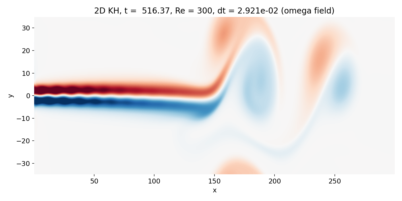
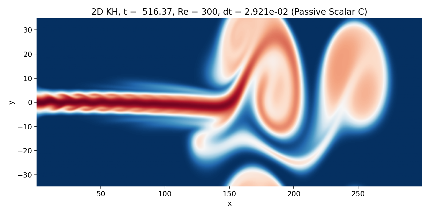
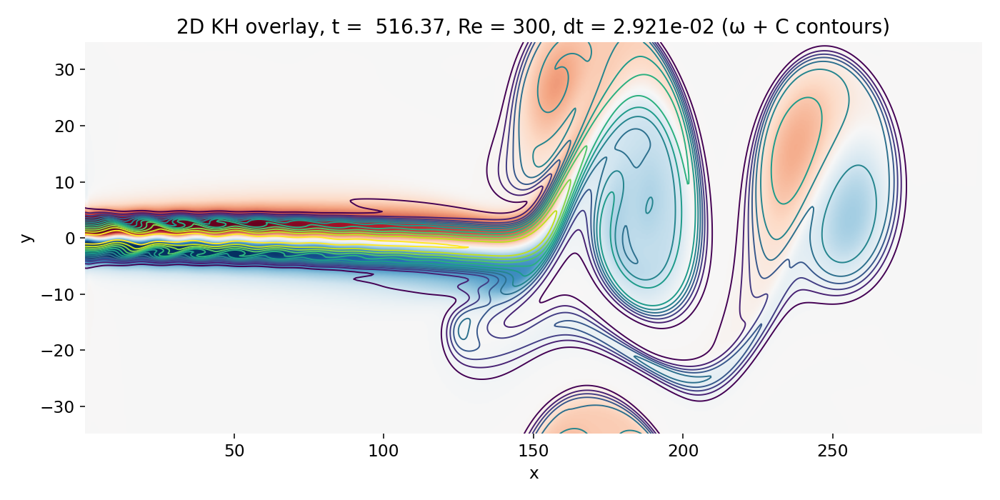
Strongly nonlinear shear layer evolution (frame 00142, $t \approx 516.4$). Large coherent vortices dominate beyond $x \gtrsim 150$, while the upstream jet remains comparatively straight and shows only weakly expressed edge waviness due to strong numerical dissipation.

The overlay again clarifies the physics: the scalar contours are not free floating decorations. They cling to the vorticity rich shear layers and then wrap around the large vortices, showing mixing and entrainment driven by rotational flow. This is the correct “KH consistency check” without adding extra diagnostics: billows in $C$ align with maxima of $|\omega|$ along the jet boundaries.

At the same time, the head vortex influence is still visible through the global jet deflection and the fact that the dominant structures are not a neat train of equally sized KH billows. Instead, the system has selected a few large structures that occupy substantial cross stream extent. That selection is consistent with vortex pairing and merger in 2D and with the head vortex imposing a large scale deformation field.

Very late time: Dominant coherent vortices and strong jet deflection

Near the end of the simulation, the flow is dominated by a few large scale coherent vortices downstream of the jet head the jet is strongly deflected. The upstream region still shows the injected jet core with relatively smooth edges, while downstream the scalar field is pulled into extended lobes and folded interfaces. The vorticity field confirms that these deformations are organized by broad vortical regions rather than by sharp, compressible features.

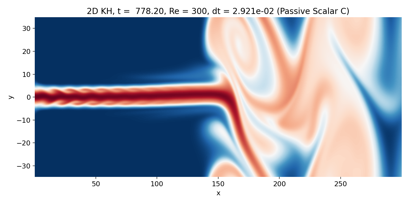
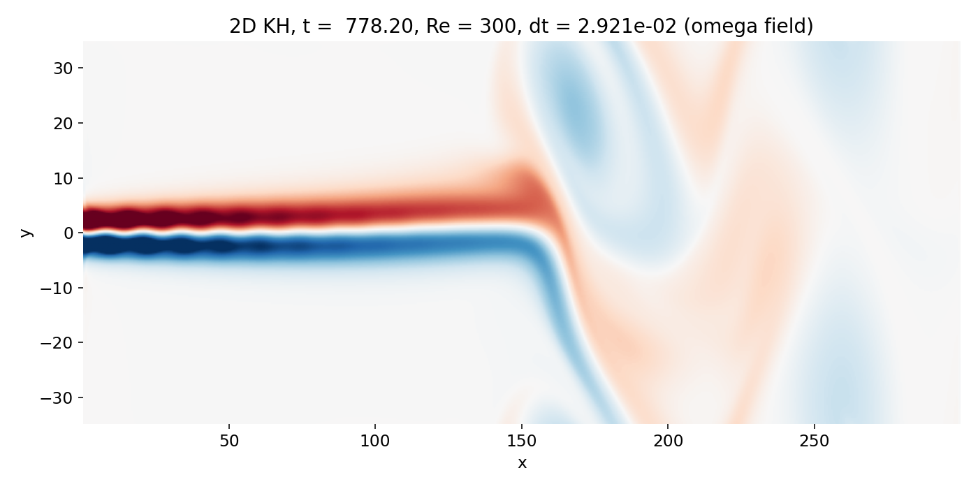
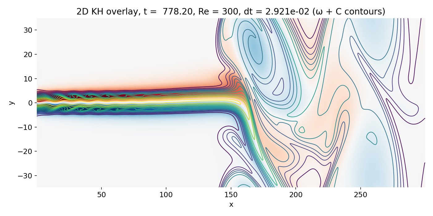
Late time regime dominated by large scale coherent vortices and strong jet deflection (frame 00214, $t \approx 778.2$). The vorticity field shows broad regions of rotation, and the scalar indicates deep entrainment and mixing along the rolled up shear layers.

A frequent temptation at this stage is to treat the sharp scalar interfaces as “fronts” analogous to compressible shocks. That interpretation remains physically incorrect here. The scalar is a passive tracer advected by an incompressible velocity field with strong numerical diffusion. Interfaces become sharp where advection compresses scalar gradients into thin layers and where contour levels cluster, but this is purely a kinematic consequence of stretching and folding plus the properties of the scheme. The correct dynamical content sits in $\omega$, which shows how shear layers roll up and how vortex induced velocities entrain ambient fluid into the jet.

Why the small edge structures look smeared

The early and small scale KH billows at the jet edges look comparatively soft for a direct reason: Numerical dissipation (most likely).

Zoomed in view of early KH billows (frame 00043, $t \approx 156.4$). The small scale edge structures appear soft due to strong numerical dissipation from the first order upwind advection scheme.

The advection operators advect_u, advect_v, and advect_scalar implement strict first order upwind. This is extremely robust, but it damps small scales aggressively. Even with $kappa = 0$ for the scalar, the scheme introduces an effective diffusivity that can be much larger than any intended physical diffusion. As a result, early KH waviness along the shear layers is smoothed and becomes visually obvious only after growth and nonlinear interaction have transferred energy into larger scales that survive the upwind damping.

What the large vortices beyond $x \gtrsim 150$ are

Beyond $x \gtrsim 150$, the flow is primarily large scale vortical dynamics of the jet shear layers. In the literature on spatially developing jets and mixing layers, these are typically described as coherent structures. In our setup, they arise from a mixture of mechanisms where Kelvin–Helmholtz roll up is central but not exclusive:

• KH roll up of the upper and lower jet shear layers. The jet has two shear layers near $y \approx \pm w$ with $w \sim \texttt{jet_w}$. Where $|\partial u/\partial y|$ is maximal, $|\omega|$ is maximal, and KH grows convectively while being advected downstream. Once nonlinear, the shear layers roll up into large vortices. The overlay frames show that the $C$ contours wrap around vorticity rich regions, consistent with this mechanism.
• Vortex pairing and merger. After the first vortices form, adjacent structures can merge into larger ones. In 2D this is particularly prominent because inverse energy transfer tends to favor growth of large scales. Visually, this corresponds to a reduction in the number of structures and growth in their size.
• Interaction with the starting jet head vortex and global jet deflection. The head vortex produces a large scale background flow that bends and stretches the shear layers. Downstream, the flow is no longer a near parallel mixing layer but a globally curved jet geometry. The observed vortices are therefore KH roll up structures evolving in a distorted background field and can look more like large lobes than like a clean periodic train.

A direct plausibility check is already embedded in the overlay: If the structures are KH related, they should sit on the shear layers and the scalar contours should wrap around vorticity concentrations. That is exactly what our plots show, especially once the large scale structures are established.

Conclusion

In this post, we explored Kelvin–Helmholtz type dynamics from a complementary numerical and physical perspective by moving from a doubly periodic, pseudospectral vorticity formulation to a finite volume projection method for the incompressible Navier–Stokes equations on a staggered grid with inflow and outflow boundaries. This change in formulation and domain setup is not merely technical. It fundamentally alters how instability growth is interpreted.

In the spatially developing jet considered here, perturbations are injected at the inlet and evolve convectively as they are transported downstream. The observed structures therefore reflect genuine downstream development rather than the artificial recirculation inherent to periodic domains. At early times, the flow is dominated by a starting jet transient. The formation of a pronounced jet head vortex is a natural consequence of accelerating a jet into quiescent fluid and must not be mistaken for compressible shock phenomena, which are excluded by construction in an incompressible formulation.

Kelvin–Helmholtz dynamics emerge along the upper and lower shear layers that bound the jet core. A central diagnostic throughout our little study was the comparison between passive scalar billows and the vorticity field. The alignment of scalar contours with regions of large vorticity magnitude provides a clear and physically grounded consistency check: Coherent billows develop where shear, and thus available kinetic energy, is maximal. This confirms that the dominant roll up structures downstream are shear driven and consistent with Kelvin–Helmholtz physics, even though their appearance is strongly influenced by the starting jet head vortex and by numerical dissipation.

The results also highlight the role of the numerical scheme. The use of first order upwind advection ensures robustness but introduces substantial numerical diffusion. As a consequence, small scale Kelvin–Helmholtz waviness near the inlet is strongly damped, and coherent billows become visually apparent only once they have grown to sufficiently large scales. Downstream, vortex pairing, merger, and interaction with the head vortex lead to a small number of dominant coherent structures, a behavior that is particularly pronounced in two dimensional flows.

Overall, this finite volume jet simulation complements our earlier spectral shear layer study by illustrating how Kelvin–Helmholtz instabilities manifest in a spatially developing setting with realistic boundary conditions. It demonstrates that interpreting flow features requires careful separation of physical mechanisms, startup transients, and numerical artifacts. In particular, sharp scalar interfaces or front like structures should not be overinterpreted as shocks, but understood as kinematic consequences of incompressible advection and shear driven vorticity dynamics.

Update and code availability: This post and its accompanying Python code were originally drafted in 2021 and archived during the migration of this website to Jekyll and Markdown. In January 2026, I substantially revised and extended the code. The updated and cleaned-up implementation is now available in this new GitHub repositoryꜛ. Please feel free to experiment with it and to share any feedback or suggestions for further improvements.

References and further reading

• Walter Greiner, Horst Stock, Hydrodynamik - Ein Lehr- und Übungsbuch; mit Beispielen und Aufgaben mit ausführlichen Lösungen, 1991, Harri Deutsch Verlag, ISBN: 9783817112043
• Heinz Schade and Ewald Kunz, Strömungslehre, 2007, de Gruyter, ISBN: 978-3-11-018972-8
• Sirovich Antman, J. E. Marsden, Hale P Holmes, J. Keller, J. Keener, B. J. Mielke, A. Matkowsky, C. S. Sreenivasan, and K. R. S. Perkin, Prandtl’s Essential of Fluid Mechanics, 2004, Vol. 158, Springer, ISBN: 0-387-40437-6
• O. G. Drazin, Introduction to hydrodynamic stability, 2002, Cambridge University Press, ISBN: 0521 80427 2
• Rutherford Aris, Vectors, tensors and the basic equations of fluid mechanics, 1962, Dover Publications Inc., ISBN: 0-486-66110-5
• Jianping Zhu, Computational Simulations and Applications, 2011, Intechweb.org, ISBN: 978-953-307-430-6
• Pieter Wesseling, Principles of computational fluid dynamics, 2001, Springer-Verlag, ISBN: 3-540-67853-0
• Franz Durst, Grundlagen der Strömungslehre, 2006, Springer-Verlag, ISBN: 978-3-540-31323-6
• Wilhelm Kley, Numerische Hydrodynamik, 2004, Universitaet Tuebingen (Lecture Notes)
• Burg, K., Haf, H., Wille, F., & Meister, A. Partielle Differentialgleichungen und funktionalanalytische Grundlagen, 2010, 5th ed., Vieweg + Teubner, ISBN: 978-3-8348-1294-0
• Lord Kelvin (William Thomson), Hydrokinetic solutions and observations, 1871, Philosophical Magazine. 42: 362–377
• Hermann von Helmholtz, Über discontinuierliche Flüssigkeits-Bewegungen [On the discontinuous movements of fluids]”, 1868, Monatsberichte der Königlichen Preussische Akademie der Wissenschaften zu Berlin. 23: 215–228
• Wikipedia article on Kelvin–Helmholtz instabilityꜛ