Hydrodynamics: A brief overview of fluid dynamics and its fundamental equations

Over the past year, I have posted a small series of articles in which we introduced key concepts from space physics. You may have noticed that many of the simulations and physical processes we discussed there have strong connections to classical fluid dynamics, both conceptually and mathematically. In a very simplified sense, for instance, we could understand magnetohydrodynamics as hydrodynamics extended by electromagnetic forces, that is, hydrodynamics with electric and magnetic fields switched on. If these additional fields are neglected, the equations reduce to those of ordinary hydrodynamics.

Example application of hydrodynamics: An inviscid, incompressible flow around an airfoil, constructed with a Joukovski transform. Levels of blue represent pressure (darkest is highest). Hydrodynamics provides the theoretical framework for understanding fluid motion in a wide range of contexts, from aerodynamics to oceanography. In this post, we explore its fundamental principles and equations. Source: Wikimedia Commonsꜛ (license: CC0 1.0 Universal).

This perspective motivated me to take a step back and look more systematically at hydrodynamics itself. In particular, I thought that it would be useful to complement the space physics series with a short sequence of posts on geophysical hydrodynamics, where many of the same ideas appear in a more familiar classical setting.

This post serves as an overview. My aim here is not to be exhaustive, but to outline what hydrodynamics is, which kinds of systems it describes, and which fundamental equations form its theoretical backbone: The continuity equation, the Navier–Stokes equation, and the energy equation.

What is fluid dynamics?

Fluid dynamics is the branch of classical physics concerned with the motion of fluids, where fluids include both liquids and gases. What distinguishes a fluid from a solid is its ability to deform continuously under applied shear stress. Rather than resisting deformation elastically, a fluid responds by flowing.

From our perspective, fluid dynamics is less a collection of isolated applications and more a unifying framework. The same underlying principles describe air flowing around an aircraft wing, ocean currents, atmospheric circulation, and the slow convection of Earth’s mantle. In geophysics, fluid dynamics is indispensable for understanding weather and climate, ocean dynamics, magma transport, and large scale energy and momentum transport within the Earth system.

The appeal of fluid dynamics lies in the fact that this wide range of phenomena can be traced back to a small set of conservation laws. Conservation of mass, momentum, and energy leads to a compact system of partial differential equations. Despite their relatively simple appearance, these equations give rise to an enormous diversity of flow behavior, from smooth laminar motion to highly irregular turbulence.

General properties of fluids

So, let’s take a closer look at fluids and their defining properties. Understanding these characteristics is essential for formulating the governing equations and for identifying the relevant physical regimes in different applications.

Viscosity

We begin with viscosity, which characterizes a fluid’s internal friction. In particular, viscosity quantifies a fluid’s resistance to deformation under shear and enters the dynamical equations through the stress tensor. For a Newtonian fluid, the viscous stress tensor $\boldsymbol{\tau}$ is linearly related to the rate of strain tensor,

\[\tau_{ij} = \mu \left( \frac{\partial u_i}{\partial x_j} + \frac{\partial u_j}{\partial x_i} \right) + \lambda \, (\nabla \cdot \mathbf{u}) \, \delta_{ij},\]

where $\mu$ is the dynamic viscosity, $\lambda$ the second viscosity coefficient, $\mathbf{u}$ the velocity field, and $\delta_{ij}$ the Kronecker delta. For incompressible flows, the divergence term vanishes and the expression simplifies considerably.

Top: A simulation of liquids with different viscosities. The liquid on the left has lower viscosity than the liquid on the right. Source: Wikimedia Commonsꜛ (license: CC BY-SA 4.0). – Bottom: Definition of viscosity: The fluid (blue) is sheared between a stationary plate (bottom) and a plate moving at velocity $v$ (top). Source: Wikimedia Commonsꜛ (license: CC BY-SA 3.0).

From a physical point of view, viscosity represents irreversible momentum transport between neighboring fluid elements. In many problems, it is useful to work with the kinematic viscosity $\nu = \mu / \rho$, which compares viscous effects directly to inertial effects. In geophysical flows, typical Reynolds numbers are often very large, indicating that viscosity mainly acts at small scales, where it ultimately dissipates kinetic energy into heat.

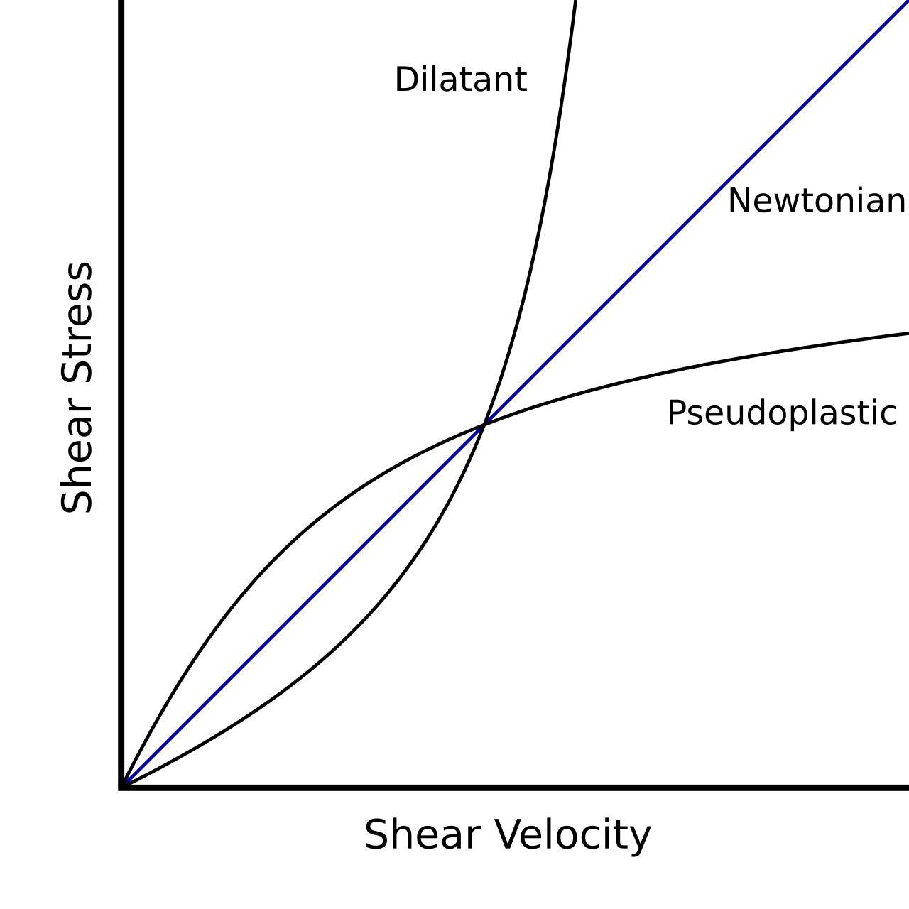
Newtonian and non-Newtonian fluids

The linear constitutive relation between stress and strain rate defines a Newtonian fluid. In this case, viscosity is a material constant independent of the flow itself. Air and water are well described by this approximation under most atmospheric and oceanic conditions.

In blue a Newtonian fluid compared to the dilatant and the pseudoplastic, angle depends on the viscosity. Source: Wikimedia Commonsꜛ (license: CC BY-SA 3.0).

Non-Newtonian fluids violate this linear relation. A common generalization replaces the constant viscosity by an effective viscosity that depends on the strain rate magnitude,

\[\mu_{\mathrm{eff}} = \mu(\dot{\gamma}),\]

where $\dot{\gamma}$ denotes a characteristic shear rate. Shear thinning fluids exhibit decreasing viscosity with increasing shear, while shear thickening fluids show the opposite behavior. In geophysical applications, ice sheets, debris flows, and partially molten rocks often require such nonlinear rheological descriptions, as their deformation cannot be captured by a constant viscosity alone.

Compressibility and sound speed

Compressibility describes how the density of a fluid responds to pressure variations. Quantitatively, it is characterized by the compressibility coefficient

\[\kappa = -\frac{1}{V} \left( \frac{\partial V}{\partial p} \right),\]

or, equivalently, through the equation of state $\rho = \rho(p, T)$. For small perturbations about an equilibrium state, compressibility gives rise to acoustic waves.

Pressure-pulse, or compression-type, wave (longitudinal wave) confined to a plane. This is the only type of sound wave that travels in fluids (gases and liquids). A pressure-type wave may also travel in solids, along with other types of waves. Source: Wikimedia Commonsꜛ (license: CC BY-SA 3.0).

The speed of sound $c_s$ is defined by

\[c_s^2 = \left( \frac{\partial p}{\partial \rho} \right)_s,\]

where the derivative is taken at constant entropy. The ratio between characteristic flow speed $U$ and sound speed defines the Mach number $M = U / c_s$. This dimensionless number determines whether compressibility effects can be neglected. In many geophysical flows, such as large scale ocean circulation, $M \ll 1$ and incompressible approximations are justified, whereas atmospheric flows and shock related phenomena require a fully compressible treatment.

Essential properties of geophysical fluids

Geophysical fluids are distinguished not only by their material properties, but also by the physical environments in which they evolve. Gravity induces density stratification, which introduces buoyancy forces proportional to density anomalies,

\[\mathbf{f}_b = - \rho' \, \mathbf{g},\]

where $\rho’$ denotes deviations from a reference density and $\mathbf{g}$ the gravitational acceleration.

In addition, geophysical flows are observed in a rotating reference frame. Rotation introduces the Coriolis force,

\[\mathbf{f}_c = -2 \rho \, \boldsymbol{\Omega} \times \mathbf{u},\]

where $\boldsymbol{\Omega}$ is the rotation vector of the Earth. The relative importance of rotation is commonly measured by the Rossby number:

\[Ro = \frac{U}{L f},\]

Stratification, rotation, and large spatial scales together lead to flow regimes that differ qualitatively from laboratory scale flows, such as quasi two dimensional turbulence and geostrophic balance.

From our perspective, these properties make geophysical fluids a particularly rich testing ground for fluid dynamics. The same fundamental equations apply, but the dominant balances between forces change, giving rise to characteristic large scale structures and long lived coherent flows.

Mathematical foundations of fluid dynamics

In the following, we summarize the fundamental equations that form the mathematical backbone of fluid dynamics. These equations emerge from the application of basic conservation laws to a continuum description of fluids. We focus on three key equations: The continuity equation, the Navier–Stokes equation, and the energy equation.

Continuity equation

The continuity equation expresses conservation of mass. In its general Eulerian form, it reads

\[\frac{\partial \rho}{\partial t} + \nabla \cdot (\rho \mathbf{u}) = 0,\]

where $\rho$ denotes the mass density and $\mathbf{u}$ the velocity field.

In fluid dynamics, we routinely switch between two complementary viewpoints. In the Eulerian description, all fields are defined at fixed positions in space and evolve in time. In the Lagrangian description, we follow individual fluid parcels along their trajectories. Compressibility enters through the divergence of the velocity field. If the density is constant, the continuity equation reduces to the incompressibility condition $\nabla \cdot \mathbf{u} = 0$.

Navier–Stokes equation

The Navier–Stokes equation encodes conservation of momentum. For a Newtonian fluid, it can be written as

\[\rho \left( \frac{\partial \mathbf{u}}{\partial t} + \mathbf{u} \cdot \nabla \mathbf{u} \right) = - \nabla p + \mu \nabla^2 \mathbf{u} + \mathbf{f},\]

where $p$ is the pressure, $\mu$ the dynamic viscosity, and $\mathbf{f}$ represents external body forces such as gravity.

This equation is the conceptual core of fluid dynamics. It balances inertia, pressure forces, viscous dissipation, and external forcing. The nonlinear advection term is responsible for much of the richness of fluid behavior, including flow instabilities and the onset of turbulence.

Energy equation

The energy equation expresses conservation of energy and couples fluid motion to thermodynamics. A common form for the internal energy per unit mass $e$ is

\[\rho \left( \frac{\partial e}{\partial t} + \mathbf{u} \cdot \nabla e \right) = - p \nabla \cdot \mathbf{u} + \Phi + \nabla \cdot (k \nabla T),\]

where $\Phi$ denotes viscous dissipation, $k$ the thermal conductivity (sometimes also denoted by $\kappa$), and $T$ the temperature.

In practice, we often work with simplified versions of the energy equation, depending on the physical regime of interest. In many geophysical applications, assumptions such as small temperature variations or near adiabatic flow lead to substantial simplifications.

Summary: The set of fluid equations

Taken together, the continuity equation, the Navier–Stokes equation, and the energy equation form a closed system once an equation of state is specified. This set of equations constitutes the mathematical foundation of classical fluid dynamics. Different limits and approximations define specialized subfields such as incompressible flow, shallow water theory, and geophysical fluid dynamics.

Overview of topics in fluid dynamics

Having introduced the fundamental concepts and governing equations, it is useful to place them into a broader thematic context. Fluid dynamics is not a single, narrowly defined discipline, but a structured collection of subfields that emphasize different physical limits, dominant forces, and characteristic flow regimes. Especially in geophysical applications, certain themes recur so frequently that they form a canonical toolbox. The following overview summarizes the main topic areas that naturally emerge from the basic equations and that will be taken up in more detail in subsequent posts.

Fundamental equations of fluid dynamics

• Continuity equation
• Navier–Stokes equation
• Energy equation
• Vorticity equation and the dynamics of rotational motion
• Potential flows and the Bernoulli equation

Navier–Stokes equations in a rotating reference frame

• Rotating reference frames and inertial forces
• Scaling analysis of the Navier–Stokes equation (including Reynolds number, Rossby number, and Mach number)
• Geostrophic balance and geostrophic wind
• Hydrothermal and buoyancy driven convection

Stratified and buoyancy-driven flows

• Stable and unstable stratification
• Buoyancy and restoring forces in density-stratified fluids
• Brunt–Väisälä frequency
• Boussinesq approximation
• Internal gravity waves

Boundary layers in geophysical flows

• Laminar and turbulent boundary layers
• Momentum and heat transport near solid boundaries
• Ekman layers in rotating systems
• Surface and bottom boundary layers in oceans and atmosphere

Waves in fluids

• Acoustic waves and compressibility effects
• Surface gravity waves
• Inertial waves in rotating fluids
• Rossby waves and large-scale planetary dynamics

Turbulence

• Turbulence as a multiscale nonlinear flow regime, including the Richardson cascade
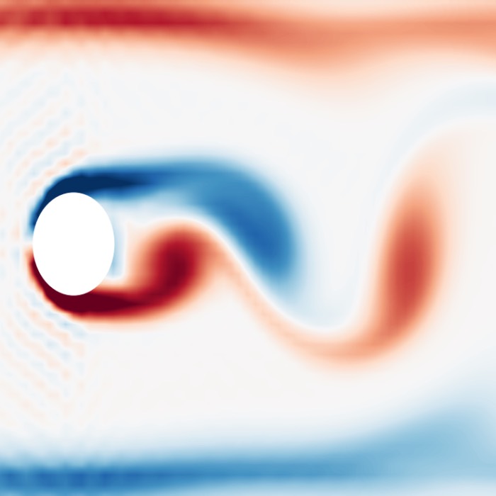
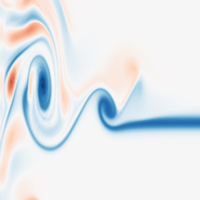
• Turbulent flows and coherent structures such as the von Kármán vortex street
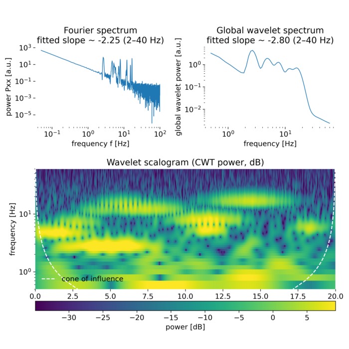
• Spectral analysis of turbulence and energy spectra
• Time–frequency analysis of turbulence and intermittency (wavelet analysis)

Reduced models in geophysical fluid dynamics

• Shallow water equations
• Quasi-geostrophic approximation
• Anelastic and pseudo-incompressible models

Summary

In this overview, we have outlined how hydrodynamics emerges from a small set of fundamental physical principles and why it is so broadly applicable. For us, hydrodynamics provides a natural bridge between classical fluid mechanics, geophysical flows, and the plasma based systems discussed in the context of space physics.

Although the governing equations are compact, their solutions exhibit remarkable complexity. Rotation, stratification, and nonlinear interactions give rise to a wide range of flow regimes that continue to be active areas of research. In the posts that follow, we will return to several of these topics in more detail and explore how hydrodynamic ideas reappear across different areas of physics.

Update and code availability: This post and its accompanying Python code were originally drafted in 2021 and archived during the migration of this website to Jekyll and Markdown. In January 2026, I substantially revised and extended the code. The updated and cleaned-up implementation is now available in this new GitHub repositoryꜛ. Please feel free to experiment with it and to share any feedback or suggestions for further improvements.

References and further reading

• Walter Greiner, Horst Stock, Hydrodynamik - Ein Lehr- und Übungsbuch; mit Beispielen und Aufgaben mit ausführlichen Lösungen, 1991, Harri Deutsch Verlag, ISBN: 9783817112043
• Heinz Schade and Ewald Kunz, Strömungslehre, 2007, de Gruyter, ISBN: 978-3-11-018972-8
• Sirovich Antman, J. E. Marsden, Hale P Holmes, J. Keller, J. Keener, B. J. Mielke, A. Matkowsky, C. S. Sreenivasan, and K. R. S. Perkin, Prandtl’s Essential of Fluid Mechanics, 2004, Vol. 158, Springer, ISBN: 0-387-40437-6
• O. G. Drazin, Introduction to hydrodynamic stability, 2002, Cambridge University Press, ISBN: 0521 80427 2
• Rutherford Aris, Vectors, tensors and the basic equations of fluid mechanics, 1962, Dover Publications Inc., ISBN: 0-486-66110-5
• Jianping Zhu, Computational Simulations and Applications, 2011, Intechweb.org, ISBN: 978-953-307-430-6
• Pieter Wesseling, Principles of computational fluid dynamics, 2001, Springer-Verlag, ISBN: 3-540-67853-0
• Franz Durst, Grundlagen der Strömungslehre, 2006, Springer-Verlag, ISBN: 978-3-540-31323-6
• Wilhelm Kley, Numerische Hydrodynamik, 2004, Universitaet Tuebingen (Lecture Notes)
• Burg, K., Haf, H., Wille, F., & Meister, A. Partielle Differentialgleichungen und funktionalanalytische Grundlagen, 2010, 5th ed., Vieweg + Teubner, ISBN: 978-3-8348-1294-0
• Lord Kelvin (William Thomson), Hydrokinetic solutions and observations, 1871, Philosophical Magazine. 42: 362–377
• Hermann von Helmholtz, Über discontinuierliche Flüssigkeits-Bewegungen [On the discontinuous movements of fluids]”, 1868, Monatsberichte der Königlichen Preussische Akademie der Wissenschaften zu Berlin. 23: 215–228
• Wikipedia article on Kelvin–Helmholtz instabilityꜛ