The von Kármán vortex street

One of the most iconic and visually striking examples of unsteady fluid flow is the von Kármán vortex street: The alternating pattern of vortices shed downstream of a bluff body such as a circular cylinder. Beyond its aesthetic appeal, the von Kármán vortex street provides a clean and well-studied setting in which to discuss instability, nonlinear saturation, and the transition from steady to unsteady flow. In this post, we first review the physical and mathematical foundations of vortex shedding and then connect them directly to a concrete numerical implementation based on the lattice–Boltzmann method.

Animation of vortex street created by a cylindrical object; the flow on opposite sides of the object is given different colors, showing that the vortices are shed from alternating sides of the object. Source: Wikimedia Commonsꜛ (license: The copyright holder (Cesareo de La Rosa Siqueira) of this file allows anyone to use it for any purpose, provided that the copyright holder is properly attributed. Redistribution, derivative work, commercial use, and all other use is permitted.).

Physical description

The von Kármán vortex street arises when a uniform flow encounters a bluff obstacle, such as a circular cylinder, at moderate Reynolds numbers. At very low Reynolds numbers, the flow remains steady and symmetric: Streamlines bend smoothly around the obstacle and rejoin downstream without forming vortices. As the Reynolds number increases, this symmetric configuration becomes unstable. Small perturbations in the wake are amplified, leading to the periodic shedding of vortices of alternating sign.

Visualisation of the vortex street behind a circular cylinder in air (on the left); the flow is made visible through release of glycerol vapour in the air near the cylinder. Source: Wikimedia Commonsꜛ (license: CC BY-SA 4.0).

Physically, this process can be understood as a competition between inertia and viscosity. The boundary layer that forms on the surface of the cylinder separates when adverse pressure gradients become sufficiently strong. Once separation occurs, the shear layers roll up into vortices. Because a perfectly symmetric shedding pattern is unstable, the system selects an alternating configuration in which vortices of opposite circulation are released on either side of the wake. The resulting pattern propagates downstream and forms the characteristic staggered street of vortices.

This phenomenon is not merely a laboratory curiosity. Vortex shedding plays an important role in engineering and geophysical contexts, including flow-induced vibrations of structures, sound generation, and wake dynamics behind islands or mountains in atmospheric and oceanic flows.

Mathematical description

From a continuum perspective, the von Kármán vortex street is a solution of the incompressible Navier–Stokes equations,

\[\begin{aligned} \nabla \cdot \mathbf{u} &= 0, \\ \frac{\partial \mathbf{u}}{\partial t} + (\mathbf{u} \cdot \nabla)\mathbf{u} &= -\frac{1}{\rho}\nabla p + \nu \nabla^2 \mathbf{u}, \end{aligned}\]

where $\mathbf{u}(\mathbf{x}, t)$ is the velocity field, $p$ the pressure, $\rho$ the density, and $\nu$ the kinematic viscosity. The Reynolds number,

\[\mathrm{Re} = \frac{U R}{\nu},\]

with characteristic velocity $U$ and length scale $R$, controls the qualitative behavior of the flow. For flow past a circular cylinder, steady solutions lose stability at Reynolds numbers of order $10^2$, giving rise to periodic vortex shedding.

A particularly useful diagnostic for this flow is the vorticity,

\[\boldsymbol{\omega} = \nabla \times \mathbf{u}.\]

In two dimensions, only the out-of-plane component $\omega_z$ is nonzero,

\[\omega_z = \frac{\partial v}{\partial x} - \frac{\partial u}{\partial y},\]

and alternating regions of positive and negative $\omega_z$ directly visualize the vortex street.

Vorticity in the numerical model

In the numerical implementation discussed below, the vorticity is computed a posteriori from the macroscopic velocity field using finite differences. This diagnostic does not enter the time integration itself but serves as a physically transparent way to identify and visualize coherent vortical structures in the wake of the cylinder.

The lattice–Boltzmann method in D2Q9 formulation

Rather than solving the Navier–Stokes equations directly, our simulation will use the so-called lattice–Boltzmann method (LBM). LBM is a mesoscopic approach in which the fluid is described by discrete distribution functions $f_i(\mathbf{x}, t)$ associated with a finite set of lattice velocities $\mathbf{c}_i$. In the D2Q9 formulation, the two-dimensional lattice is equipped with nine discrete velocities,

6   2   5
  \ | /
3 - 0 - 1
  / | \
7   4   8

At each lattice node, the macroscopic density and velocity are recovered as moments of the distribution functions,

\[\begin{aligned} \rho &= \sum_i f_i, \\ \mathbf{u} &= \frac{1}{\rho} \sum_i f_i \mathbf{c}_i. \end{aligned}\]

The equilibrium distribution functions are given by a low-Mach-number expansion of the Maxwell–Boltzmann distribution,

\[f_i^{\mathrm{eq}} = \rho w_i \left[ 1 + 3 (\mathbf{c}_i \cdot \mathbf{u}) + \frac{9}{2} (\mathbf{c}_i \cdot \mathbf{u})^2 - \frac{3}{2} |\mathbf{u}|^2 \right],\]

where $w_i$ are lattice-dependent weights.

Time evolution proceeds through a collision and streaming process. In the BGK (Bhatnagar–Gross–Krook) approximation, the collision step relaxes the distributions toward equilibrium,

\[f_i \leftarrow f_i - \omega (f_i - f_i^{\mathrm{eq}}),\]

with relaxation factor $\omega$. The streaming step shifts the post-collision distributions along the lattice velocities. In the low-Mach-number limit, this scheme reproduces the Navier–Stokes equations with kinematic viscosity

\[\nu = \frac{1}{3}\left(\frac{1}{\omega} - \frac{1}{2}\right).\]

Although LBM formally solves a weakly compressible system, keeping the Mach number sufficiently small ensures that density fluctuations remain minor and the flow behaves effectively incompressibly.

Numerical implementation

The numerical experiment considered here simulates two-dimensional flow past a circular cylinder in a channel using the D2Q9 lattice–Boltzmann method described above. The implementation follows a classical inflow–outflow configuration with a no-slip obstacle and is designed as a transparent reference model for visualization and didactic purposes.

The computational domain is discretized into a Cartesian grid of size $(N_x, N_y)$, with nine distribution functions stored at each lattice node. The left boundary enforces a uniform inflow velocity profile using a Zou–He velocity boundary condition. At the right boundary, a simple outflow condition is applied by copying left-moving populations from the interior. The top and bottom boundaries are treated as no-slip walls via bounce-back, forming a channel. The circular obstacle representing a two-dimensional slice of a cylinder also enforces a no-slip boundary condition through bounce-back.

The fluid is initialized with a uniform horizontal velocity field throughout the domain. To trigger vortex shedding, a small localized perturbation in the vertical velocity component is introduced downstream of the cylinder. Time integration then proceeds by iterating the following steps:

1. Apply the outflow boundary condition.
2. Compute macroscopic density and velocity.
3. Impose the inflow profile using the Zou–He formulation.
4. Compute equilibrium distribution functions.
5. Perform the BGK collision step.
6. Apply bounce-back boundary conditions at walls and obstacle.
7. Stream the distributions along the lattice velocities.
8. Advance to the next time step.

Our implementation is basically a NumPy-based version of Felix Köhlerꜛ’s lattice–Boltzmann method tutorialꜛ, which uses JAX for array operations and automatic differentiation. Here, we reimplement the algorithm using standard NumPy to make the code a little more accessible and easier to follow for readers unfamiliar with JAX. However, the core algorithmic structure and numerical scheme remain essentially the same and I thank Felix for making his code publicly available under MIT license.

So, let’s begin by importing the necessary libraries:

import os
import numpy as np
import matplotlib.pyplot as plt
import imageio.v2 as imageio
from tqdm import tqdm

In the first step, we define simulation parameters and create an output folder for saving frames. We set a moderate number of iterations of 15,000 and a Reynolds number of 80, which is known to produce a clear von Kármán vortex street. The domain size, cylinder position, and radius are chosen to ensure sufficient resolution of the flow features:

N_ITERATIONS = 25_000
REYNOLDS_NUMBER = 80

N_POINTS_X = 300
N_POINTS_Y = 50

CYLINDER_CENTER_INDEX_X = N_POINTS_X // 5
CYLINDER_CENTER_INDEX_Y = N_POINTS_Y // 2
CYLINDER_RADIUS_INDICES = N_POINTS_Y // 9

MAX_HORIZONTAL_INFLOW_VELOCITY = 0.04

VISUALIZE = True
PLOT_EVERY_N_STEPS = 100
SKIP_FIRST_N_ITERATIONS = 0000

MAKE_GIF = True
GIF_PATH = f"von_karman_numpy_Re{REYNOLDS_NUMBER}.gif"
GIF_FPS = 20

RANDOM_SEED = 1

# create output folder for frames:
FRAMES_PATH = f"frames_Re{REYNOLDS_NUMBER}"
os.makedirs(FRAMES_PATH, exist_ok=True)

Next, we define the lattice setup, including the discrete velocities, their opposites, and the associated weights. We also predefine index arrays for convenience in applying boundary conditions later on:

N_DISCRETE_VELOCITIES = 9

# velocities as (cx, cy) per direction i:
LATTICE_VELOCITIES = np.array(
    [
        [0, 0],   # 0
        [1, 0],   # 1
        [0, 1],   # 2
        [-1, 0],  # 3
        [0, -1],  # 4
        [1, 1],   # 5
        [-1, 1],  # 6
        [-1, -1], # 7
        [1, -1],  # 8
    ],
    dtype=int
)

OPPOSITE_LATTICE_INDICES = np.array([0, 3, 4, 1, 2, 7, 8, 5, 6], dtype=int)

LATTICE_WEIGHTS = np.array(
    [
        4/9,
        1/9, 1/9, 1/9, 1/9,
        1/36, 1/36, 1/36, 1/36,
    ],
    dtype=float)

RIGHT_VELOCITIES = np.array([1, 5, 8], dtype=int)
UP_VELOCITIES = np.array([2, 5, 6], dtype=int)
LEFT_VELOCITIES = np.array([3, 6, 7], dtype=int)
DOWN_VELOCITIES = np.array([4, 7, 8], dtype=int)

PURE_VERTICAL_VELOCITIES = np.array([0, 2, 4], dtype=int)
PURE_HORIZONTAL_VELOCITIES = np.array([0, 1, 3], dtype=int)

We then implement several helper functions to create the cylinder mask, compute macroscopic density and velocity, calculate equilibrium distribution functions, and evaluate vorticity:

def make_cylinder_mask(nx: int, ny: int, cx: int, cy: int, r: int) -> np.ndarray:
    """ 
    Create a boolean mask for a cylinder in a 2D grid.
    """
    x = np.arange(nx)[:, None]
    y = np.arange(ny)[None, :]
    return (x - cx) ** 2 + (y - cy) ** 2 < r ** 2

def get_density(f: np.ndarray) -> np.ndarray:
    """ 
    Compute macroscopic density from distribution functions.
    """
    return np.sum(f, axis=-1)

def get_macroscopic_velocities(f: np.ndarray, rho: np.ndarray) -> np.ndarray:
    """ 
    Compute macroscopic velocities from distribution functions and density.
    """
    jx = np.sum(f * LATTICE_VELOCITIES[None, None, :, 0], axis=-1)
    jy = np.sum(f * LATTICE_VELOCITIES[None, None, :, 1], axis=-1)
    u = np.zeros((f.shape[0], f.shape[1], 2), dtype=float)
    u[..., 0] = jx / rho
    u[..., 1] = jy / rho
    return u

def get_equilibrium_discrete_velocities(u: np.ndarray, rho: np.ndarray) -> np.ndarray:
    """ 
    Compute equilibrium distribution functions for given macroscopic velocities and density.
    """
    ux = u[..., 0]  # (nx, ny)
    uy = u[..., 1]  # (nx, ny)

    # cu = c_i · u:
    cu = (
        LATTICE_VELOCITIES[None, None, :, 0] * ux[..., None]
        +
        LATTICE_VELOCITIES[None, None, :, 1] * uy[..., None]
    )  # (nx, ny, 9)

    uu = ux**2 + uy**2  # (nx, ny)

    feq = (
        rho[..., None]
        * LATTICE_WEIGHTS[None, None, :]
        * (1.0 + 3.0 * cu + 4.5 * cu**2 - 1.5 * uu[..., None]))
    
    return feq

def compute_vorticity(u: np.ndarray) -> np.ndarray:
    """ 
    Compute the z-component of the vorticity (curl) of a 2D velocity field.
    
    u shape: (nx, ny, 2). We compute curl_z = d u_y / d x - d u_x / d y
    """
    dux_dx, dux_dy = np.gradient(u[..., 0], axis=(0, 1))
    duy_dx, duy_dy = np.gradient(u[..., 1], axis=(0, 1))
    return (duy_dx - dux_dy)

Having all necessary components in place, we proceed to set up the simulation. We initialize the random number generator for perturbations, compute the relaxation parameter based on the desired Reynolds number, and create masks for the cylinder obstacle and channel walls:

# setup random number generator:
rng = np.random.default_rng(RANDOM_SEED)

# this follows the logic of the JAX code:
# nu = (U_max * R) / Re
# omega = 1 / (3 nu + 0.5)
kinematic_viscosity = (MAX_HORIZONTAL_INFLOW_VELOCITY * CYLINDER_RADIUS_INDICES) / REYNOLDS_NUMBER
relaxation_omega = 1.0 / (3.0 * kinematic_viscosity + 0.5)

# domain mask:
obstacle_mask = make_cylinder_mask(
    N_POINTS_X, N_POINTS_Y,
    CYLINDER_CENTER_INDEX_X, CYLINDER_CENTER_INDEX_Y,
    CYLINDER_RADIUS_INDICES)

# create wall masks (top and bottom):
wall_mask = np.zeros((N_POINTS_X, N_POINTS_Y), dtype=bool)
wall_mask[:, 0] = True
wall_mask[:, -1] = True

solid_mask = obstacle_mask | wall_mask

We then define the inflow velocity profile and initialize the distribution functions to equilibrium. A small perturbation is added downstream of the cylinder to break symmetry and trigger vortex shedding:

# inflow profile u(x=0, y, :) prescribed for y=1:-1:
velocity_profile = np.zeros((N_POINTS_X, N_POINTS_Y, 2), dtype=float)
velocity_profile[:, :, 0] = MAX_HORIZONTAL_INFLOW_VELOCITY
velocity_profile[:, :, 1] = 0.0

We also initialize the distribution functions to equilibrium based on the uniform inflow:

# initialize distributions to equilibrium of uniform inflow:
rho0 = np.ones((N_POINTS_X, N_POINTS_Y), dtype=float)
u0 = velocity_profile.copy()
u0[solid_mask, :] = 0.0
f = get_equilibrium_discrete_velocities(u0, rho0)

To initiate vortex shedding, we introduce a small random perturbation in the vertical velocity component just downstream of the cylinder:

# small perturbation near cylinder to break symmetry:
x0 = CYLINDER_CENTER_INDEX_X + CYLINDER_RADIUS_INDICES + 2
x1 = min(N_POINTS_X, x0 + 30)
y0 = max(1, CYLINDER_CENTER_INDEX_Y - 10)
y1 = min(N_POINTS_Y - 1, CYLINDER_CENTER_INDEX_Y + 10)
u0[x0:x1, y0:y1, 1] += 1e-4 * (rng.random((x1 - x0, y1 - y0)) - 0.5)
f = get_equilibrium_discrete_velocities(u0, rho0)

Our final step is the main simulation loop, where we iterate through the time steps, applying boundary conditions, computing macroscopic fields, performing collision and streaming, and visualizing the results at specified intervals:

frames_rgb = []
for iteration_index in tqdm(range(N_ITERATIONS)):
    f_prev = f

    # (1) outflow BC at right boundary: copy left-moving populations from x = -2 to x = -1:
    f_prev[-1, :, LEFT_VELOCITIES] = f_prev[-2, :, LEFT_VELOCITIES]

    # (2) Macroscopic fields
    rho = get_density(f_prev)
    u = get_macroscopic_velocities(f_prev, rho)

    # enforce no-slip in macroscopic fields on solids (helps diagnostics and stability):
    u[solid_mask, :] = 0.0

    # (3) Zou/He velocity inlet at x=0 for y=1:-1:
    u[0, 1:-1, :] = velocity_profile[0, 1:-1, :]

    # reconstruct inlet density (same formula as in the JAX code):
    # rho_in = (sum f_i over pure vertical + 2 sum f_i over left movers) / (1 - u_x)
    f0 = f_prev[0, :, :]                  # shape should be (ny, 9)
    sum_pure_vertical = f0[:, PURE_VERTICAL_VELOCITIES].sum(axis=1)  # (ny,)
    sum_left = f0[:, LEFT_VELOCITIES].sum(axis=1)                    # (ny,)
    rho_in = (sum_pure_vertical + 2.0 * sum_left) / (1.0 - u[0, :, 0])
    rho[0, :] = rho_in

    # walls at inlet should remain no-slip:
    u[0, 0, :] = 0.0
    u[0, -1, :] = 0.0

    # (4) equilibrium:
    feq = get_equilibrium_discrete_velocities(u, rho)

    # (3b) Zou/He completion: set right-moving populations at inlet from equilibrium
    f_prev[0, :, RIGHT_VELOCITIES] = feq[0, :, RIGHT_VELOCITIES]

    # (5) BGK collision:
    f_post = f_prev - relaxation_omega * (f_prev - feq)

    # (6) bounce-back on solids, using pre-collision populations as in the JAX version:
    for i in range(N_DISCRETE_VELOCITIES):
        f_post[solid_mask, i] = f_prev[solid_mask, OPPOSITE_LATTICE_INDICES[i]]

    # (7) streaming (periodic roll in x and y):
    # walls block physical wrap-around through bounce-back, but the roll is convenient and standard.
    f_stream = f_post.copy()
    for i in range(N_DISCRETE_VELOCITIES):
        cx, cy = LATTICE_VELOCITIES[i]
        f_stream[:, :, i] = np.roll(np.roll(f_post[:, :, i], shift=cx, axis=0), shift=cy, axis=1)

    f = f_stream

    # diagnostics for blow-up:
    if iteration_index % 200 == 0:
        rho_chk = get_density(f)
        if not np.isfinite(rho_chk).all():
            print(f"Non-finite density at iteration {iteration_index}. Aborting.")
            break

    # plotting:
    if VISUALIZE and iteration_index % PLOT_EVERY_N_STEPS == 0 and iteration_index > SKIP_FIRST_N_ITERATIONS:
        rho_vis = get_density(f)
        u_vis = get_macroscopic_velocities(f, rho_vis)
        u_vis[solid_mask, :] = 0.0

        speed = np.linalg.norm(u_vis, axis=-1)
        vort = compute_vorticity(u_vis)

        fig = plt.figure(figsize=(15, 6))

        ax1 = plt.subplot(211)
        im1 = ax1.contourf(
            speed.T,
            levels=50,
            cmap="viridis")
        plt.colorbar(im1, ax=ax1).set_label("velocity magnitude")
        ax1.add_patch(
            plt.Circle(
                (CYLINDER_CENTER_INDEX_X, CYLINDER_CENTER_INDEX_Y),
                CYLINDER_RADIUS_INDICES,
                color="white",
                zorder=5))
        ax1.set_xticks([])
        ax1.set_yticks([])
        ax1.set_title(f"speed, iter={iteration_index}, Re≈{REYNOLDS_NUMBER}")

        ax2 = plt.subplot(212)
        """ im2 = ax2.contourf(
            vort.T,
            levels=50,
            cmap="RdBu_r",
            vmin=-0.02,
            vmax=0.02,
        )
        plt.colorbar(im2, ax=ax2).set_label("vorticity (curl z)") """
        im2 = ax2.imshow(
            vort.T,
            origin="lower",
            cmap="RdBu_r",
            vmin=-0.02,
            vmax=0.02,
            interpolation="bilinear",
            aspect="auto")
        plt.colorbar(im2, ax=ax2).set_label("vorticity (curl z)")
        ax2.add_patch(
            plt.Circle(
                (CYLINDER_CENTER_INDEX_X, CYLINDER_CENTER_INDEX_Y),
                CYLINDER_RADIUS_INDICES,
                color="white",
                zorder=5))
        ax2.set_xticks([])
        ax2.set_yticks([])
        ax2.set_title("vorticity")

        plt.tight_layout()

        # render figure to RGB array (in-memory):
        fig.canvas.draw()
        buf = np.asarray(fig.canvas.buffer_rgba())
        rgb = buf[:, :, :3].copy()   # drop alpha channel

        if MAKE_GIF:
            frames_rgb.append(rgb)

        # also save current frame as PNGs for inspection:
        frame_path = os.path.join(FRAMES_PATH, f"frame_{iteration_index:05d}.png")
        plt.savefig(frame_path, dpi=300)

        plt.close(fig)

if MAKE_GIF and len(frames_rgb) > 0:
    imageio.mimsave(GIF_PATH, frames_rgb, fps=GIF_FPS)
    print(f"Saved GIF to: {GIF_PATH}")

Discussion of the simulation results

The numerical experiments presented here illustrate the emergence and evolution of a von Kármán vortex street in a controlled and progressively more complex manner. By combining time-resolved animations with carefully selected snapshots and parameter sweeps in the Reynolds number, our simulation allows a direct connection between classical fluid-dynamical theory and its numerical realization within the Lattice–Boltzmann framework.

Time-resolved evolution at Re $\approx$ 80

At Re $\approx$ 80, the simulation exhibits a canonical von Kármán vortex street. After an initial adjustment phase, the wake behind the cylinder becomes unstable to transverse perturbations and starts shedding vortices of alternating sign. These vortices are convected downstream while maintaining a remarkably regular spacing and amplitude, indicating a fully developed laminar vortex street rather than turbulent breakdown.

Temporal evolution of the flow field at Reynolds number Re $\approx$ 80. The upper panel shows the velocity magnitude, while the lower panel displays the vorticity field. After an initial transient, a stable and periodic vortex shedding pattern develops downstream of the cylinder.

The velocity magnitude highlights the accelerating flow around the cylinder flanks and the low-velocity recirculation region in the near wake. The vorticity field, in contrast, provides a much clearer diagnostic of the underlying dynamics: The alternating red and blue structures correspond to coherent vortices with opposite circulation, whose periodic release defines the shedding frequency.

Developmental stages at Re $\approx$ 80

In order to get a better understanding of the vortex shedding process, we examine three representative snapshots at different iterations during the simulation at Re $\approx$ 80.

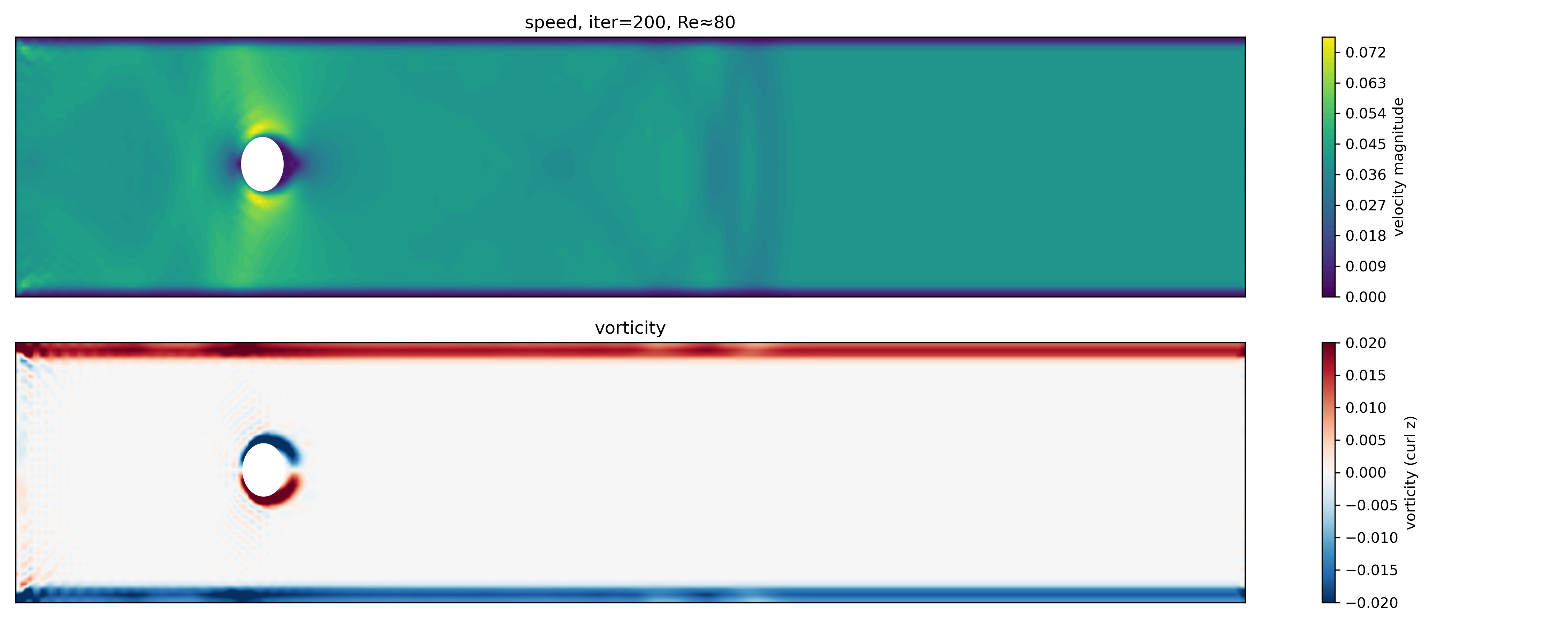Iteration 200 (Re $\approx$ 80): Onset of the simulation, before vortex shedding has developed.

At iteration 200, the flow is still dominated by a symmetric wake. A steady recirculation bubble forms immediately behind the cylinder, but no alternating vortex shedding is present yet. The vorticity is concentrated near the cylinder surface and along the channel walls, reflecting boundary-layer formation rather than global instability.

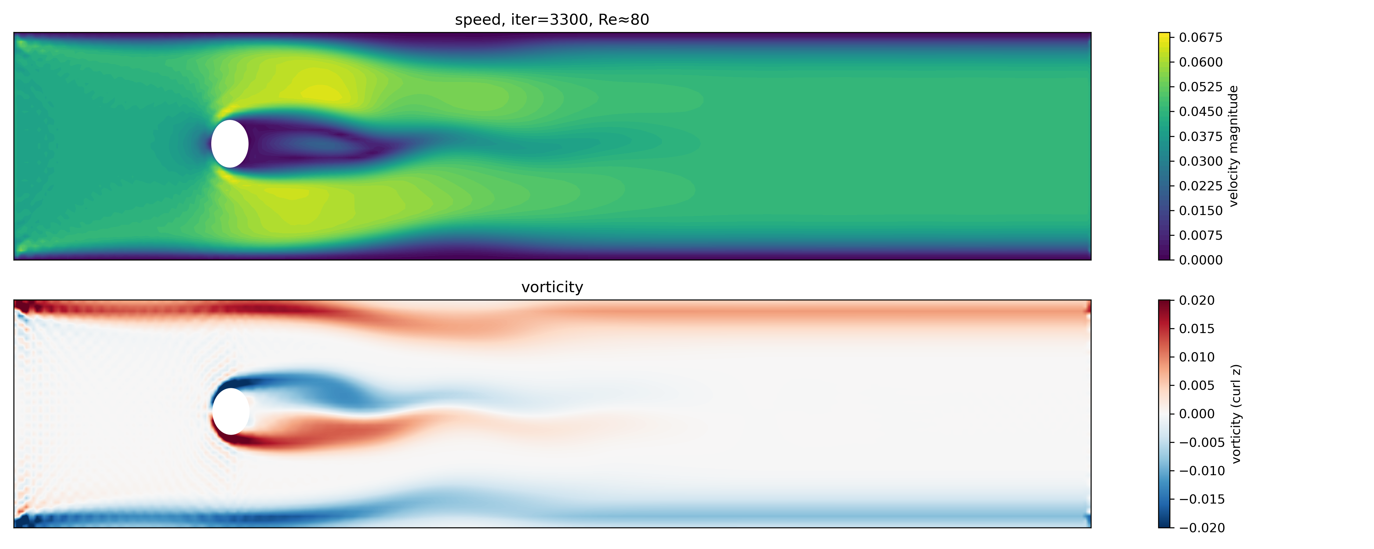Iteration 3300 (Re $\approx$ 80): Initial appearance of alternating vortices in the wake.

By iteration 3300, the wake symmetry has broken. The first alternating vortices appear close to the cylinder, indicating the onset of the Hopf-type instability associated with the von Kármán street. The downstream region still shows remnants of the earlier symmetric flow, illustrating that vortex shedding develops locally and then propagates downstream.

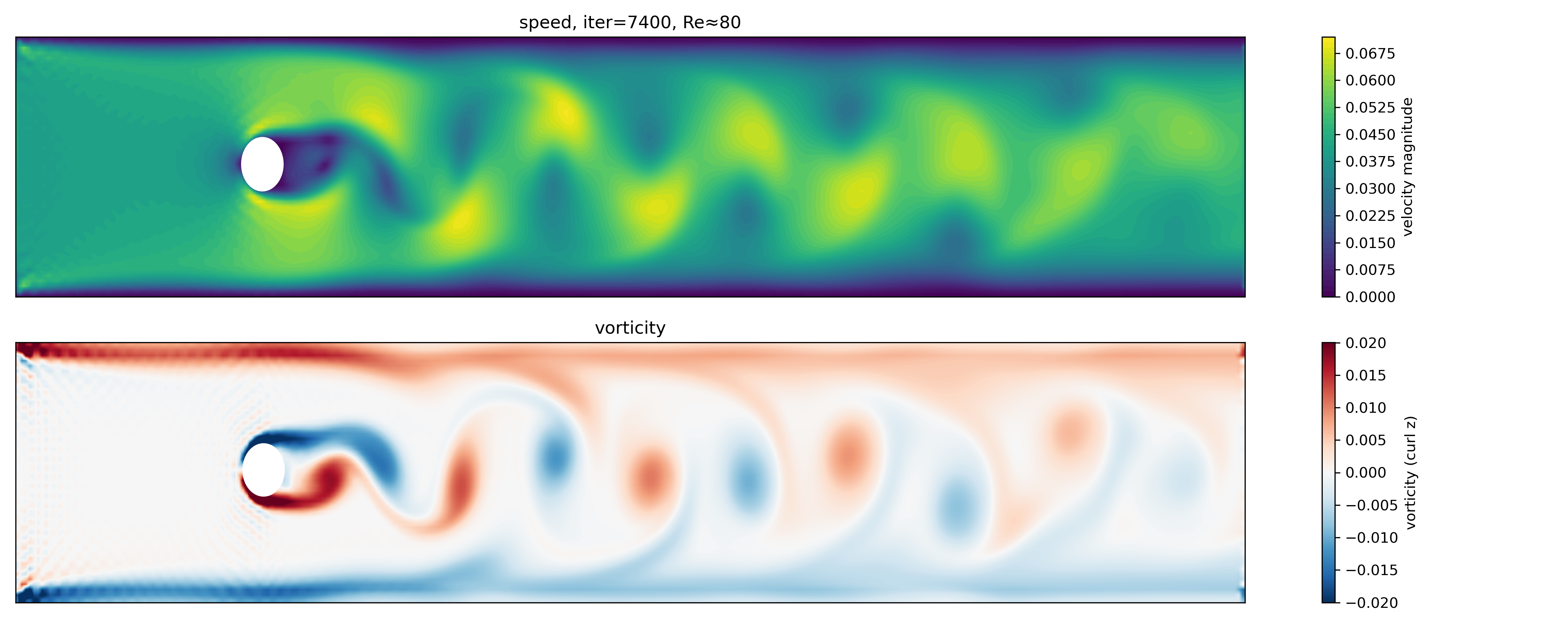
Iteration 7400 (Re $\approx$ 80): Fully developed vortex shedding. The wake has reached a statistically stationary state characterized by periodic, alternating vortices with nearly constant wavelength and amplitude.

At iteration 7400, the flow has reached a quasi-steady regime in which vortex shedding is fully developed and temporally periodic. The spacing between vortices and the width of the wake remain approximately constant, consistent with classical experimental observations for laminar cylinder wakes in this Reynolds number range.

Dependence on the Reynolds number

Appert from Re $\approx$ 80, I have also performed simulations at several other Reynolds numbers to illustrate the transition from steady laminar flow to periodic vortex shedding.

Re $\approx$ 4

At Re $\approx$ 4, the flow remains steady and symmetric. No vortex shedding occurs; the wake consists of a smooth, stationary recirculation region.

In this low-Reynolds-number regime, viscous forces dominate over inertia. The flow is laminar, steady, and time-independent, corresponding to the classical Stokes or creeping-flow regime.

Re $\approx$ 30

At Re $\approx$ 30, a steady but elongated wake forms. The flow remains symmetric, but the recirculation zone grows in length, indicating proximity to the instability threshold.

Here, inertial effects become more important, but the flow is still below the critical Reynolds number for time-dependent vortex shedding. The wake lengthens, and the system becomes increasingly sensitive to perturbations.

Re $\approx$ 35

At Re $\approx$ 35, the wake shows intermittent unsteadiness and weak asymmetries. This regime is close to the critical Reynolds number for the onset of periodic vortex shedding.

The flow begins to exhibit time-dependent behavior, but the vortex street is not yet fully developed. Small perturbations can grow transiently before being damped, reflecting marginal stability.

Re $\approx$ 40

At Re $\approx$ 40, sustained and periodic vortex shedding emerges. The wake clearly transitions from a steady to an oscillatory state.

This Reynolds number marks the effective onset of the von Kármán vortex street in the present numerical configuration. The critical value is consistent with classical results for two-dimensional cylinder flows, taking into account numerical diffusion and finite domain effects.

High-Reynolds-number regime

To explore the behavior at higher Reynolds numbers, I also conducted a simulation at Re $\approx$ 300.

At Re $\approx$ 300, vortex shedding becomes stronger and less regular. While a von Kármán-like pattern is still visible, the wake shows increased complexity and signs of secondary instabilities.

In this regime, the limitations of a two-dimensional BGK-LBM become apparent. The flow exhibits larger velocity gradients and more complex vorticity structures, approaching conditions where three-dimensional effects and turbulence would dominate in real fluids. Nevertheless, the simulation still captures the essential qualitative transition from laminar vortex shedding toward more chaotic wake dynamics.

Summary of our findings

Overall, these results demonstrate that the implemented LBM scheme reproduces the classical sequence of wake regimes behind a circular cylinder: steady laminar flow at low Reynolds numbers, the onset of periodic vortex shedding near a critical threshold, and increasingly complex unsteady behavior at higher Reynolds numbers.

Conclusion

In this post, we examined the von Kármán vortex street as a prototypical example of flow instability in fluid dynamics and used it as a test case for a Python-based implementation of the Lattice–Boltzmann method in D2Q9 formulation. Incorporating the essential physical ingredients and boundary conditions, we simulated two-dimensional flow past a circular cylinder over a range of Reynolds numbers and analyzed the resulting wake dynamics.

The numerical results reproduce the classical sequence of wake regimes behind a circular cylinder. At low Reynolds numbers, the flow remains steady and symmetric, dominated by viscous effects. As the Reynolds number is increased, the wake elongates and approaches a marginally stable state. Beyond a critical Reynolds number, periodic vortex shedding emerges through a symmetry-breaking instability, giving rise to a well-defined von Kármán vortex street. At even higher Reynolds numbers, the wake becomes increasingly complex and less regular, indicating the limitations of a two-dimensional, weakly compressible BGK–LBM in capturing fully developed turbulent dynamics.

From a methodological perspective, the simulations highlight the strengths of the lattice–Boltzmann approach as an exploratory tool. The method provides a conceptually simple route from microscopic distribution functions to macroscopic flow behavior, while still capturing subtle instability mechanisms such as vortex shedding. At the same time, the results make clear where care is required: Stability is controlled primarily by the Mach number rather than the Reynolds number, boundary condition choices strongly influence wake development, and truly turbulent regimes would require three-dimensional modeling and more advanced collision operators.

Overall, the von Kármán vortex street serves as an ideal benchmark for both physical understanding and numerical experimentation. The implementation we used here demonstrates that even a compact, readable code can recover key features of classical fluid dynamics, making it well suited for demonstrations purposes, but also for qualitative studies, and it a good starting point for more advanced extensions such as three-dimensional flows, improved collision models, or quantitative comparisons with experimental data.

At the end, I’d like to thank again Felix Köhlerꜛ for sharing his JAX-based implementation of the lattice–Boltzmann method, which served as the basis for this NumPy reimplementation.

Update info (Jan 2026): Please note that this post was initially without an accompanying code implementation and archived during the migration of this website to Jekyll in 2021. Meanwhile, I found an excellent reference implementation of the lattice–Boltzmann method in JAXꜛ by Felix Köhlerꜛ, which I reimplemented in standard NumPy to make it more accessible. In Januar 2026, I revised the original post and added the new code implementation. The updated is available in this new GitHub repositoryꜛ. Please feel free to experiment with it and to share any feedback or suggestions for further improvements.

References and further reading

• Walter Greiner, Horst Stock, Hydrodynamik - Ein Lehr- und Übungsbuch; mit Beispielen und Aufgaben mit ausführlichen Lösungen, 1991, Harri Deutsch Verlag, ISBN: 9783817112043
• Heinz Schade and Ewald Kunz, Strömungslehre, 2007, de Gruyter, ISBN: 978-3-11-018972-8
• Sirovich Antman, J. E. Marsden, Hale P Holmes, J. Keller, J. Keener, B. J. Mielke, A. Matkowsky, C. S. Sreenivasan, and K. R. S. Perkin, Prandtl’s Essential of Fluid Mechanics, 2004, Vol. 158, Springer, ISBN: 0-387-40437-6
• O. G. Drazin, Introduction to hydrodynamic stability, 2002, Cambridge University Press, ISBN: 0521 80427 2
• Rutherford Aris, Vectors, tensors and the basic equations of fluid mechanics, 1962, Dover Publications Inc., ISBN: 0-486-66110-5
• Jianping Zhu, Computational Simulations and Applications, 2011, Intechweb.org, ISBN: 978-953-307-430-6
• Pieter Wesseling, Principles of computational fluid dynamics, 2001, Springer-Verlag, ISBN: 3-540-67853-0
• Franz Durst, Grundlagen der Strömungslehre, 2006, Springer-Verlag, ISBN: 978-3-540-31323-6
• Wilhelm Kley, Numerische Hydrodynamik, 2004, Universitaet Tuebingen (Lecture Notes)
• Burg, K., Haf, H., Wille, F., & Meister, A. Partielle Differentialgleichungen und funktionalanalytische Grundlagen, 2010, 5th ed., Vieweg + Teubner, ISBN: 978-3-8348-1294-0
• Lord Kelvin (William Thomson), Hydrokinetic solutions and observations, 1871, Philosophical Magazine. 42: 362–377
• Hermann von Helmholtz, Über discontinuierliche Flüssigkeits-Bewegungen [On the discontinuous movements of fluids]”, 1868, Monatsberichte der Königlichen Preussische Akademie der Wissenschaften zu Berlin. 23: 215–228
• Lewis Fry Richardson, Weather Prediction by Numerical Process, 1922, Cambridge University Press, ISBN: 9780521680448, archive.orgꜛ
• Kolmogorov, A. N., The local structure of turbulence in incompressible viscous fluid for very large Reynolds numbers, 1890, Vol. 434, No. 1890, Turbulence and Stochastic Process: Kolmogorov’s Ideas 50 Years On (Jul. 8, 1991), pp. 9-13, online PDFꜛ
• Frisch, U., Turbulence: the legacy of A. N. Kolmogorov, 1995/2010, Cambridge University Press, ISBN: 978-0521457132
• Pope, S. B., Turbulent flows, 2000, Cambridge University Press, ISBN: 978-0521598866
• Davidson, P. A., Turbulence: an introduction for scientists and engineers, 2015, Oxford University Press, ISBN: 978-0198722595
• Koehler, F., Machine Learning and Simulation, Computer software, DOI: 10.5281/zenodo.12793323ꜛ, GitHub: Ceyron/machine-learning-and-simulationꜛ