Step-by-step NEST single neuron simulation

While NEST is designed for large-scale simulations of neural spike networks, the underlying models are based on approximating the behavior of single neurons and synapses. Before using NEST for network simulations, it is probably helpful to first understand the basic functions of the software tool by modelling and studying the behavior of individual neurons. In this tutorial, you will learn about NEST’s concept of nodes and connections, how to set up a neuron model of your choice, how to change model parameters, which different stimulation paradigms are included in NEST and how to record and analyze the simulation results.

A single neuron simulated with with the iaf_psc_alpha model (leaky integrate-and-fire model with alpha-shaped input currents) with an input current of 376.0 pA in NEST.

Getting started

Installation

NEST can be easily installedꜛ via conda:

conda create -n nest -y python=3.11
conda activate nest
conda install -c conda-forge mamba
mamba install -c conda-forge ipykernel matplotlib numpy pandas scipy nest-simulator

Windows users: Unfortunately, NEST is not supported on Windows. However, you can try to use the Windows Subsystem for Linux (WSL)ꜛ to run NEST on your Windows machine.

Importing NEST

In your script, simply import the nest module via import nest. It is recommended to import any additionally required modules, such as numpy, matplotlib, scipy, or sklearn, before importing nest to avoid any potential conflicts:

import numpy as np
import matplotlib.pyplot as plt
import nest

Nodes and connections

A typical NEST network consists of two main components: nodes and connections. A node is either a neuron, a device or even a sub-network. A connection is a directed link between two nodes. Devices are used to inject current into and stimulate neurons or to record data from them.

Creating a node

Let’s begin by creating our first node, a single neuron. First, choose one of the many neuron modelsꜛ available in NEST. For this example, we will use the iaf_psc_alphaꜛ neuron model, which is a simple leaky integrate-and-fire neuron with an alpha-shaped postsynaptic current. With nest.Create(model, n=1, params=None, positions=None)ꜛ, we create a single neuron of this type:

neuron = nest.Create('iaf_psc_alpha')

List all available models: You can list all available neuron and synapse models in NEST by using the nest.Models() function. Detailed information about each model can be obtained from the corresponding model documentationꜛ.

By default, a single neuron is created unless n is further specified. The neuron is created with a predefined set of parameters. The params argument can be used to create a neuron with specific parameters. For example, to create a neuron with a membrane potential of -70 mV, a threshold of -55 mV, and a reset potential of -70 mV, we can use:

neuron = nest.Create('iaf_psc_alpha', params={'V_m': -70.0, 'V_th': -55.0, 'V_reset': -70.0})

To review the parameters of the neuron and their currently set values, we can use the get() function,

neuron.get()

To retrieve specific parameters, we can specify the key of the parameter we are interested in, e.g.,

print(neuron.get("I_e"))
neuron.get(["V_reset", "V_th"])

You can change the parameters of the neuron by using the set() function at any time, e.g.:

neuron.set("I_e": 376.0)
neuron.set({"V_reset": -70.0, "V_th": -55.0})

Another way to retrieve and change parameters is to address them directly, e.g.:

neuron.I_e
neuron.I_e = 376.0

NEST is type sensitive: If a parameter is set to a wrong type, e.g., float, NEST will raise an error if you try to set it to an int.

Creating recording devices

Recording devicesꜛ are used to collect or sample observables from the simulation such as membrane potentials, spike times, or conductances. NEST comes with a variety of recording devices, such as

• multimeterꜛ: records various analog values from neurons
• voltmeterꜛ: a pre-configured multimeter, that records the membrane potential V_m of a neuron
• spike_recorderꜛ: records the spiking events produced by a neuron
• weight_recorderꜛ: records the synaptic weights of a connection

They can be created again by using the nest.Create() function, e.g.:

multimeter = nest.Create("multimeter")
multimeter.set(record_from=["V_m"])
spikerecorder = nest.Create("spike_recorder")

For the multimeter, we need to specify the observables we want to record. In this case, we record the membrane potential V_m. A sampling interval (default is 1.0 ms) can be set either by providing the corresponding argument while creating the device,

multimeter = nest.Create("multimeter",  {'interval': 0.1, 'record_from': ['V_m', 'g_ex']})

or by using the SetStatus() function:

multimeter = nest.Create("multimeter")
multimeter.SetStatus({'interval': 0.1, 'record_from': ['V_m', 'g_ex']})

Note that we also provided the record_from in the handed-over parameter dictionary. It is very important to note, that the set of variables to record from and the recording interval must be set before the multimeter is connected to the neuron. These properties cannot be changed afterwards.

Recording devices can receive further parameters such as

• n_events: number of events that were collected by the recorder can be read out of the n_events entry.
• start and stop: start and stop time of the recording in ms, relative to origin.
• record_to: defines the recording backend (default: memory).

The record_to argument is quite interesting as it allows you to specify the recording backend, for which you can select from:

• memoryꜛ: writes data to the memory (default)
• asciiꜛ: writes data to plain text files
• screenꜛ: writes data to the terminal
• sionlibꜛ: writes data to a file in the SIONlib formatꜛ (an efficient binary format)
• mpiꜛ: sends data with MPI

Changed the recording backend from the default (memory) to a file-based backend can become important when you, e.g., run large-scale simulations and want to avoid memory overflows.

Specific neuron models come with specific parameters that can be recorded. To get a list of all recordable parameters, you can use the GetDefaults() function:

nest.GetDefaults(neuron.model)['recordables']

Connecting nodes

Now that we have created one node for the neuron and two nodes for the recording devices, we can connect them. To connect two nodes, we use the nest.Connect()ꜛ function, which connects a pre-node to a post-node. Before we do so, it is important to understand that there is a fundamental difference between samplers and collectors recording devices. Samplers are recording devices that actively communicate with their target nodes at given time intervals (e.g., to record membrane potentials). Collectors, in contrast, are recording devices, that gather events sent to them (e.g., spikes). It matters in which order or direction you connect them to the nodes: collectors are connected to the neuron(s), while neuron(s) are connected to the samplers:

nest.Connect(multimeter, neuron)
nest.Connect(neuron, spikerecorder)

The order specified in the nest.Connect() command reflects the actual flow of events: If the neuron spikes, it sends an event to the spike recorder (collector), while the multimeter (sampler) periodically sends requests to the neuron to ask for its membrane potential at that point in time.

Without further specifications, a default connection paradigm is used. However, you can specify the connection parameters, such as the synaptic weight, the delay, or the connection rule. Since this starts becoming relevant when you work with networks with more than one neuron (population), we will not go into detail here and refer to the next post, where we will discuss multi-neuron network simulations.

Connecting neurons to each other: Of cause, you can also connect neurons to each otherꜛ. This is done in the same way as connecting a neuron to a recording device.

Simulating the network

After setting up the network, we can finally simulate it by using the nest.Simulate() function. This function takes the simulation time in milliseconds as an argument:

nest.Simulate(1000.0)

And that’s it! By executing this command, NEST will simulate the network and records the defined observables for the subsequent analysis.

Extracting and plotting the recorded data

After the simulation is finished, you can retrieve the recorded data from the recording devices via the get() function:

recorded_events = multimeter.get()
recorded_V = recorded_events["events"]["V_m"]
time       = recorded_events["events"]["times"]
spikes     = spikerecorder.get("events")
senders    = spikes["senders"]

You can now plot time vs. recorded_V and time vs. senders to visualize the membrane potential and the spike times, respectively:

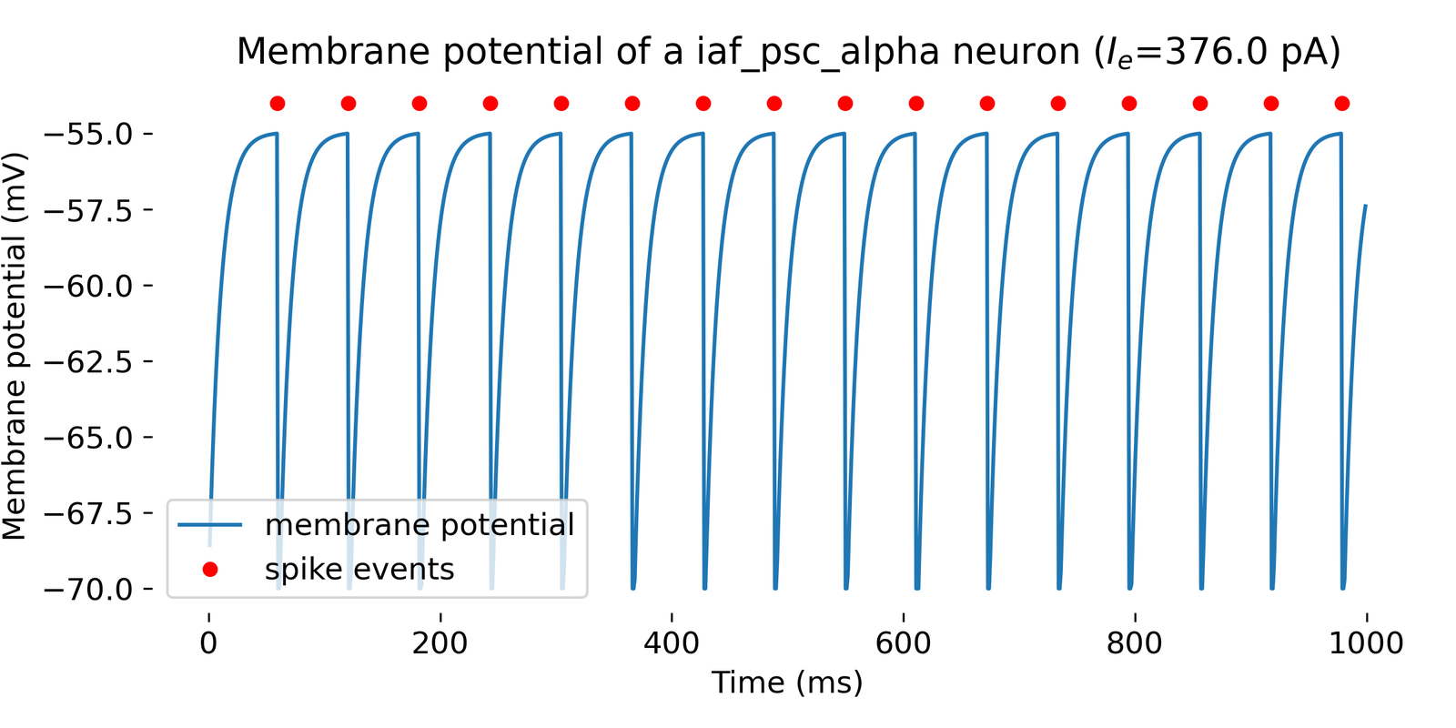Simulation results of a single neuron with the iaf_psc_alpha model and an input current of 376.0 pA. The membrane potential is plotted over time, and the red dots indicate the spike events. The neuron spikes at a membrane potential of -55 mV. The simulation was run for 1000 ms.

The corresponding plot commands are provided in the next subsection, where the entire simulation script is presented.

Putting it all together

Here is the complete simulation code including all settings made above:

import matplotlib.pyplot as plt
import numpy as np
from pprint import pprint
import nest

# set the verbosity of the NEST simulator:
nest.set_verbosity("M_WARNING")

# reset the kernel for safety:
nest.ResetKernel()

# list all available models:
pprint(nest.Models())

# create the neuron, a spike recorder and a multimeter (all called "nodes"):
neuron     = nest.Create("iaf_psc_alpha")
multimeter = nest.Create("multimeter")
multimeter.set(record_from=["V_m"]) 
spikerecorder = nest.Create("spike_recorder")

pprint(neuron.get())
pprint(f"I_e: {neuron.get('I_e')}")
pprint(f"V_reset: {neuron.get('V_reset')}")
pprint(f"{neuron.get(['V_m', 'V_th'])}")

neuron.set({"V_reset": -70.0})
pprint(f"{neuron.get('V_reset')}")

# set a constant input current for the neuron:
I_e = 376.0 # [pA]
neuron.I_e = I_e # [pA]
pprint(f"{neuron.get('I_e')}")

# list all recordable quantities
pprint(f"recordables of {neuron.model}: {nest.GetDefaults(neuron.model)['recordables']}")

# now, connect the nodes:
nest.Connect(multimeter, neuron)
nest.Connect(neuron, spikerecorder)

# run a simulation for 1000 ms:
nest.Simulate(1000.0)

# extract recorded data from the multimeter and plot it:
recorded_events = multimeter.get()
recorded_V = recorded_events["events"]["V_m"]
time = recorded_events["events"]["times"]
spikes = spikerecorder.get("events")
senders = spikes["senders"]

plt.figure(figsize=(8, 4))
plt.plot(time, recorded_V, label="membrane potential")
plt.plot(spikes["times"], spikes["senders"]+np.max(recorded_V), "r.", markersize=10,
         label="spike events")
plt.xlabel("Time (ms)")
plt.ylabel("Membrane potential (mV)")
plt.title(f"Membrane potential of a {neuron.get('model')} neuron ($I_e$={I_e} pA)")
plt.gca().spines["top"].set_visible(False)
plt.gca().spines["bottom"].set_visible(False)
plt.gca().spines["left"].set_visible(False)
plt.gca().spines["right"].set_visible(False)
plt.legend(loc="lower left")
plt.tight_layout()
plt.show()

Note that we additionally set the verbosity of the NEST simulator to M_WARNING to suppress any unnecessary output. Also, we reset the kernel at the beginning of the script (nest.ResetKernel()) to ensure that we start with a clean slate.

Changing the stimulation paradigm

In the above example, we used a constant input current to stimulate the neuron, that was defined by the parameter I_e. However, NEST offers a variety of other stimulation devicesꜛ:

• ac_generator: produces an alternating current (AC) input
• dc_generator: provides a direct current (DC) input
• step_current_generator: provides a piecewise constant DC input current
• noise_generator: generates a Gaussian white noise current
• poisson_generator: generates spikes with Poisson process statistics
• spike_generator: generates spikes from an array with spike-times
• spike_train_injector: neuron that emits prescribed spike trains

These devices can be created as any other device in NEST with the nest.Create() function. For instance, here is how to create a poisson_generator to stimulate the neuron with a Poisson process:

neuron     = nest.Create("iaf_psc_alpha")
noise      = nest.Create("poisson_generator")
multimeter = nest.Create("multimeter")
multimeter.set(record_from=["V_m", "I_syn_ex", "I_syn_in"])
spikerecorder = nest.Create("spike_recorder")

In order to see just the effect of the Poisson process on the neuron, we should ensure that the neuron is not stimulated by any other external input current:

neuron.I_e = 0.0
pprint(f"I_e: {neuron.get('I_e')}")

We can further specify the average firing rate (spikes/s) of the Poisson generator by setting the rate parameter:

noise.rate = 68000.0 # [Hz]

Also for stimulation devices, you can set the start and stop parameters to define the time interval in which the device is active. See the documentation of the respective device for further details.

We further adjust the parameters of our IaF model to generate some spikes and to play around with later:

# change the membrane time constant:
nest.SetStatus(neuron, {"tau_m": 11}) # [ms], default is 10 ms

# change the spike threshold:
nest.SetStatus(neuron, {"V_th": -55.0}) # [mV], default is -55 mV

By increasing the membrane time constant tau_m, the neuron will integrate the input current over a longer time period, i.e., the neuron will be more sensitive to the input current and will fire more easily. A decrease of the spike threshold V_th will let the neuron fire more easily, i.e., the neuron fires more often and at lower input currents.

We need to connect the Poisson generator to the neuron and run the simulation:

nest.Connect(multimeter, neuron)
nest.Connect(noise, neuron)
nest.Connect(neuron, spikerecorder)

nest.Simulate(1000.0)

This time, we also extract the excitatory and inhibitory synaptic input currents from the multimeter to see how the injected Poisson current looks like:

recorded_events = multimeter.get()
recorded_V = recorded_events["events"]["V_m"]
time = recorded_events["events"]["times"]
spikes = spikerecorder.get("events")
senders = spikes["senders"]
recorded_current_ex = recorded_events["events"]["I_syn_ex"] # Excitatory synaptic input current
recorded_current_in = recorded_events["events"]["I_syn_in"] # Inhibitory synaptic input current

Here are the corresponding simulations results:

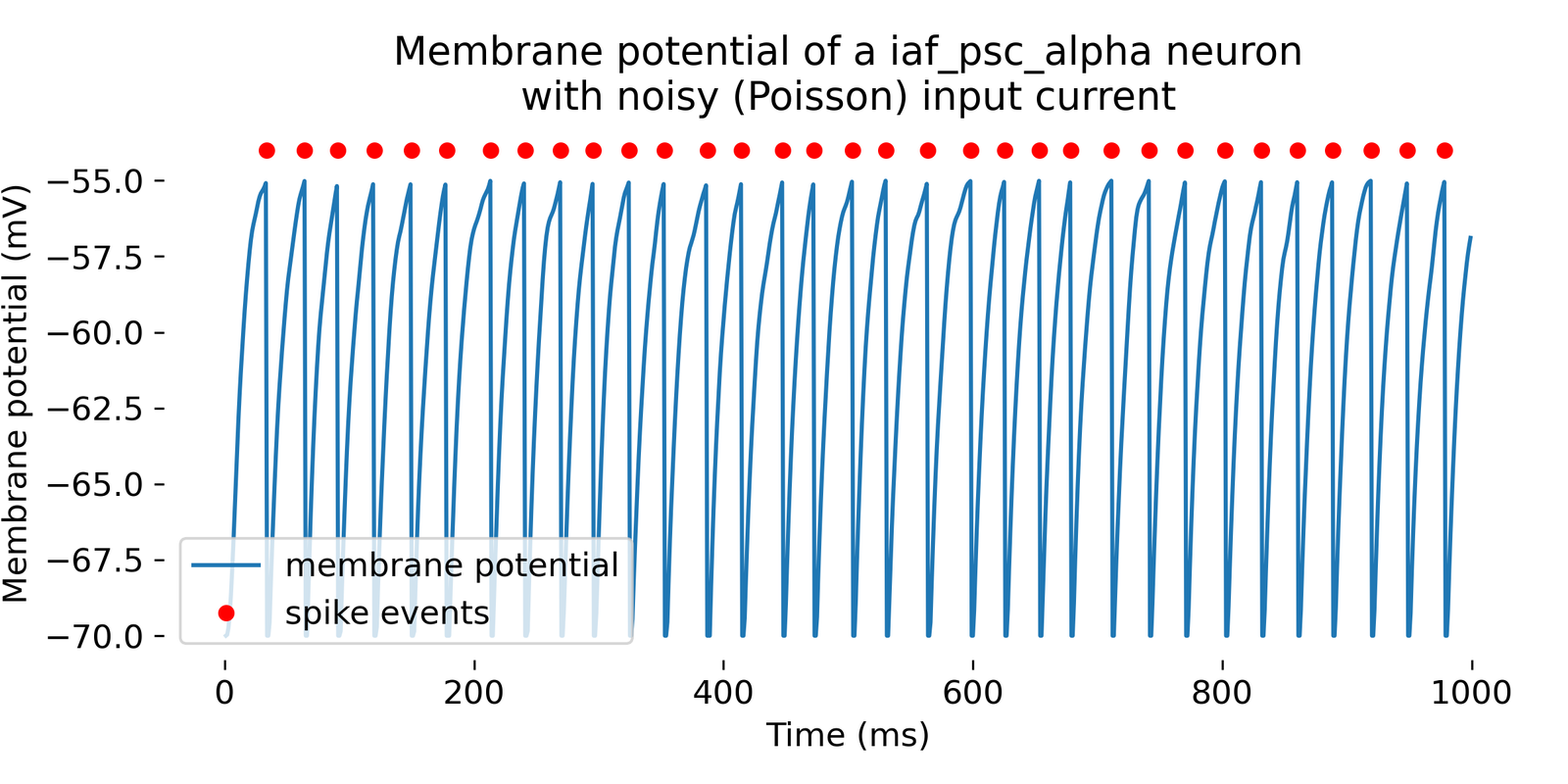
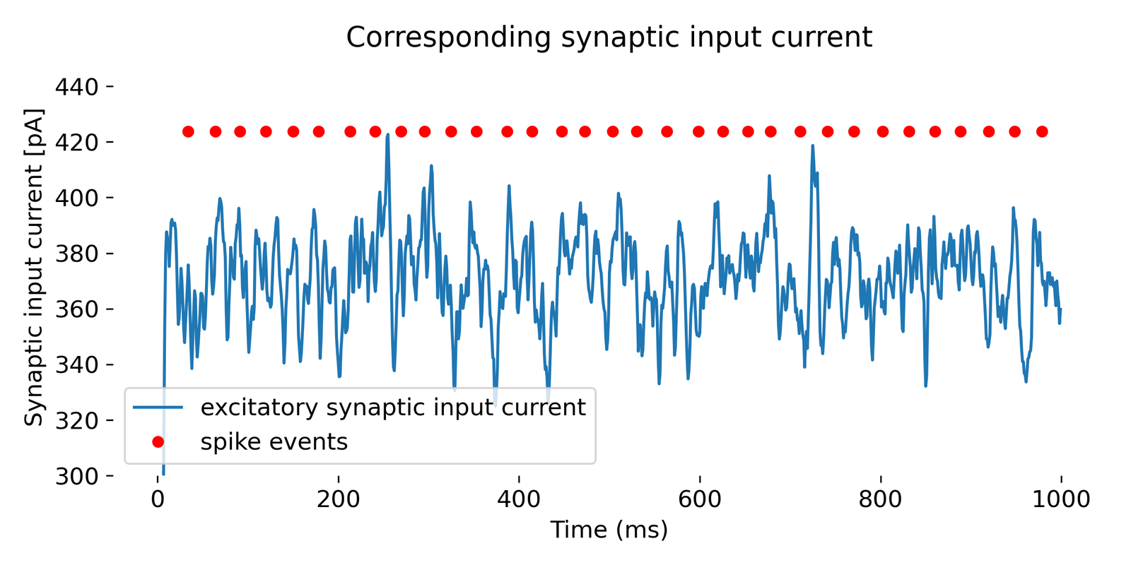Simulation of a iaf_psc_alpha neuron with a Poisson generator as input. In the upper panel, we see again the membrane potential over time, and in the lower panel, we see additionally the excitatory synaptic input currents (inhibitory synaptic input currents are zero). The simulation was run for 1000 ms.

By increasing the mean firing rate of the Poisson generator to, e.g., 88,000 Hz, the neuron will fire more often:

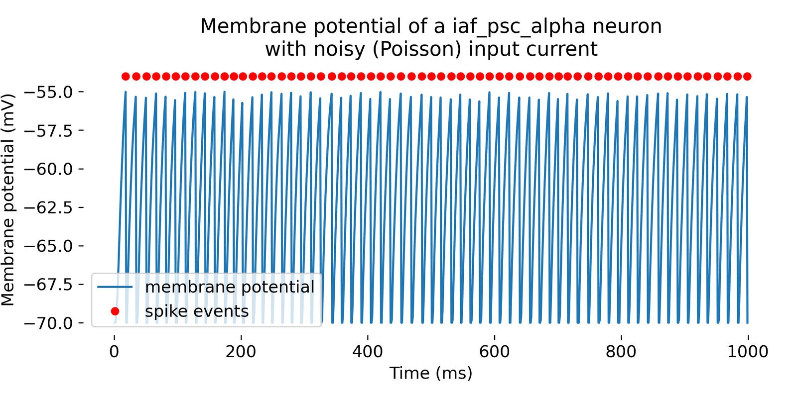
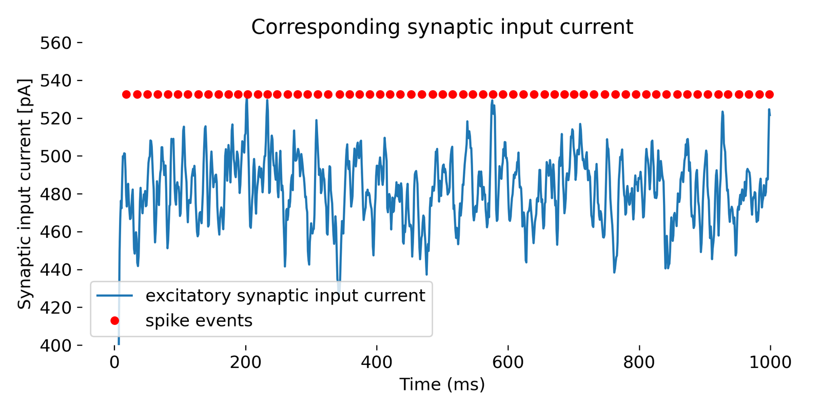Same simulation as above, but with a higher mean firing rate of the Poisson generator (88,000 Hz). The neuron fires more often and at lower input currents. The simulation was run for 1000 ms.

You may have noticed that the firing rate of the Poisson generator does not directly translate into the firing rate of the neuron. This is because the neuron integrates the input current over time, and the firing rate of the neuron depends on the actual input current and the neuron’s parameters such as the firing threshold or the membrane time constant. Regarding the input current, the noise.rate parameter in the poisson_generator indeed sets the mean rate of the Poisson process used to generate spikes. On average, spikes are generated at this rate, but due to the stochastic nature of the process, the actual number of spikes in any given second can vary.

Another factor affecting the actual spike frequency are the connections weights. So far, we have used default connection parameters and we will further discuss different connection paradigms in the next post. However, the synaptic weight of the connection between the poisson_generator and the neuron determines how much each spike affects the neuron’s membrane potential. Higher weights mean each spike has a greater effect, potentially leading to more frequent firing if the integrated input reaches the threshold more often.

In summary, setting a high noise.rate does not mean that the neuron will fire at that rate. Instead, it means that the neuron will receive a high rate of synaptic inputs, which then interact with the neuron’s properties to determine its actual firing rate. Feel free to play around with the example above and change the noise.rate as well as the neuron’s parameters to see how they affect the actual spiking behavior of the neuron.

Using NEST for studying model dynamics

With NEST, it is very easy to study the behavior of neuron models under changing conditions. For instance, we can simulate the Hodgkin-Huxley model by using the hh_psc_alpha neuron modelꜛ:

# define the neuron model and recording devices:
neuron     = nest.Create("hh_psc_alpha")
multimeter = nest.Create("multimeter")
multimeter.set(record_from=["V_m"])
spikerecorder = nest.Create("spike_recorder")

# set a constant input current for the neuron:
I_e = 650.0 # [pA] # 630.0: spike train; 620.0: a few spikes; 360.0: single spike
neuron.I_e = I_e # [pA]
pprint(f"{neuron.get('I_e')}")

# connect the nodes:
nest.Connect(multimeter, neuron)
nest.Connect(neuron, spikerecorder)

# run a simulation for 200 ms:
nest.Simulate(200.0)

# extract recorded data:
recorded_events = multimeter.get()
recorded_V = recorded_events["events"]["V_m"]
time       = recorded_events["events"]["times"]
spikes     = spikerecorder.get("events")
senders    = spikes["senders"]

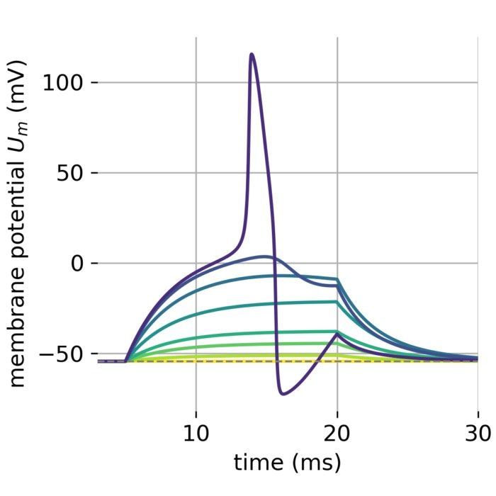
For different input currents, we trigger different responses of the neuron model:

• for an input current of 360 pA, the neuron fires a single spike
• for an input current of 620 pA, the neuron fires a few spikes
• for input currents above 630 pA, the neuron fires a spike train

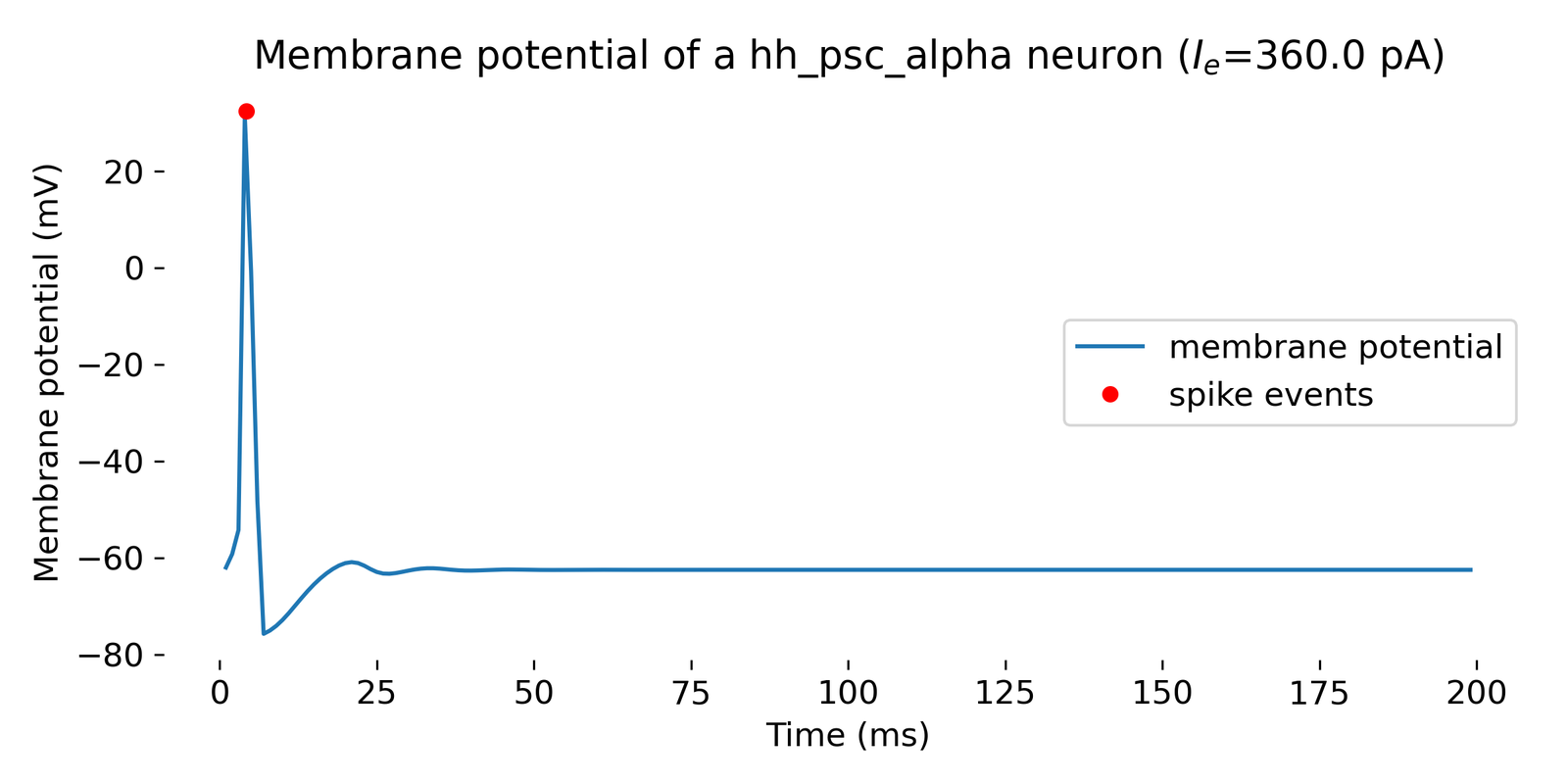
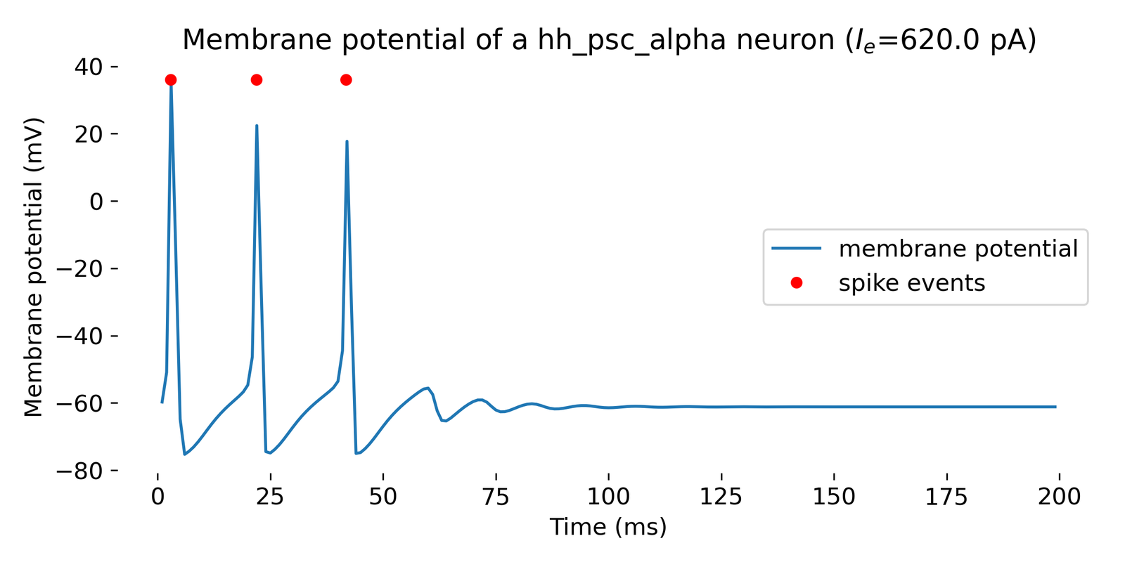
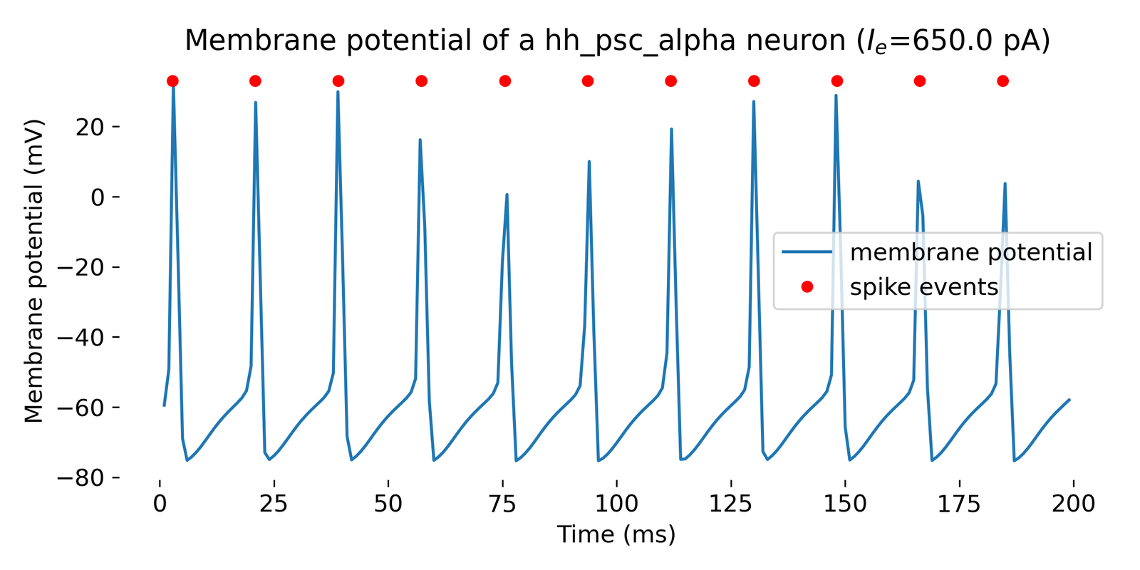Simulation of a Hodgkin-Huxley model neuron for an input current of $I_e=$ 360 pA (single spike, upper panel), 620 pA (a few spikes, middle panel), and 650 pA (spike train, lower panel). The simulation was run for 200 ms.

You can further play around with the parameters of the neuron model such as by changing the membrane capacitance, the leak conductances, or several other parameters of the Hodgkin-Huxley model.

Create individual model copies

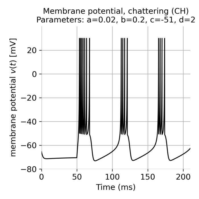
Sometimes, you may want to study a neuron model under different conditions, e.g., with different parameters or different initial conditions. In this case, you can create a copy of the model and adjust the parameters of the copy. This can be achieved with the nest.CopyModel()ꜛ command, which creates a copy of a given model with the specified parameters and adds it to the current model zoo. To demonstrate this, let’s recap the Izhikevich neuron model from the previous post with its different typical parameters to generate different firing patterns:

# define sets of typical parameters of the Izhikevich neuron model:
p_RS  = [0.02, 0.2, -65, 8, "regular spiking (RS)"] # regular spiking settings for excitatory neurons (RS)
p_IB  = [0.02, 0.2, -55, 4, "intrinsically bursting (IB)"] # intrinsically bursting (IB)
p_CH  = [0.02, 0.2, -51, 2, "chattering (CH)"] # chattering (CH)
p_FS  = [0.1, 0.2, -65, 2, "fast spiking (FS)"] # fast spiking (FS)
p_TC  = [0.02, 0.25, -65, 0.05, "thalamic-cortical (TC)"] # thalamic-cortical (TC) (doesn't work well)
p_LTS = [0.02, 0.25, -65, 2, "low-threshold spiking (LTS)"] # low-threshold spiking (LTS)
p_RZ  = [0.1, 0.26, -65, 2, "resonator (RZ)"] # resonator (RZ)

We now create a copy of the original NEST izhikevichꜛ model for each parameter set:

nest.CopyModel("izhikevich", "izhikevich_RS", {"a": p_RS[0], "b": p_RS[1], "c": p_RS[2], "d": p_RS[3]})
nest.CopyModel("izhikevich", "izhikevich_IB", {"a": p_IB[0], "b": p_IB[1], "c": p_IB[2], "d": p_IB[3]})
nest.CopyModel("izhikevich", "izhikevich_CH", {"a": p_CH[0], "b": p_CH[1], "c": p_CH[2], "d": p_CH[3]})
nest.CopyModel("izhikevich", "izhikevich_FS", {"a": p_FS[0], "b": p_FS[1], "c": p_FS[2], "d": p_FS[3]})
nest.CopyModel("izhikevich", "izhikevich_TC", {"a": p_TC[0], "b": p_TC[1], "c": p_TC[2], "d": p_TC[3]})
nest.CopyModel("izhikevich", "izhikevich_LTS", {"a": p_LTS[0], "b": p_LTS[1], "c": p_LTS[2], "d": p_LTS[3]})
nest.CopyModel("izhikevich", "izhikevich_RZ", {"a": p_RZ[0], "b": p_RZ[1], "c": p_RZ[2], "d": p_RZ[3]})

You can verify that the models have been created by listing all available models:

pprint(nest.Models())

Note, that your custom models are not saved permanently. If you restart the kernel, the default NEST model zoo is restored.

Now, let’s simulate and plot all different model variants:

model_loop_list = ["izhikevich_RS", "izhikevich_IB", "izhikevich_CH", "izhikevich_FS", "izhikevich_TC", "izhikevich_LTS", "izhikevich_RZ"]

for model in model_loop_list:
    # create the neuron, a spike recorder and a multimeter:
    neuron     = nest.Create(model)
    multimeter = nest.Create("multimeter")
    multimeter.set(record_from=["V_m"])
    spikerecorder = nest.Create("spike_recorder")
    
    # set a constant input current for the neuron:
    I_e = 10.0 # [pA]
    neuron.I_e = I_e # [pA]

    # now, connect the nodes:
    nest.Connect(multimeter, neuron)
    nest.Connect(neuron, spikerecorder)

    # run a simulation for 1000 ms:
    nest.Simulate(1000.0)

    # extract recorded data from the multimeter and plot it:
    recorded_events = multimeter.get()
    recorded_V = recorded_events["events"]["V_m"]
    time       = recorded_events["events"]["times"]
    spikes     = spikerecorder.get("events")
    senders    = spikes["senders"]

    plt.figure(figsize=(8, 4))
    plt.plot(time, recorded_V, label="membrane potential")
    plt.plot(spikes["times"], spikes["senders"]+np.max(recorded_V), "r.", markersize=10,
            label="spike events")
    plt.xlabel("Time (ms)")
    plt.ylabel("Membrane potential (mV)")
    plt.title(f"Membrane potential of a {neuron.get('model')} neuron ($I_e$={I_e} pA)")
    plt.gca().spines["top"].set_visible(False)
    plt.gca().spines["bottom"].set_visible(False)
    plt.gca().spines["left"].set_visible(False)
    plt.gca().spines["right"].set_visible(False)
    plt.legend(loc="center right")
    plt.tight_layout()
    plt.show()

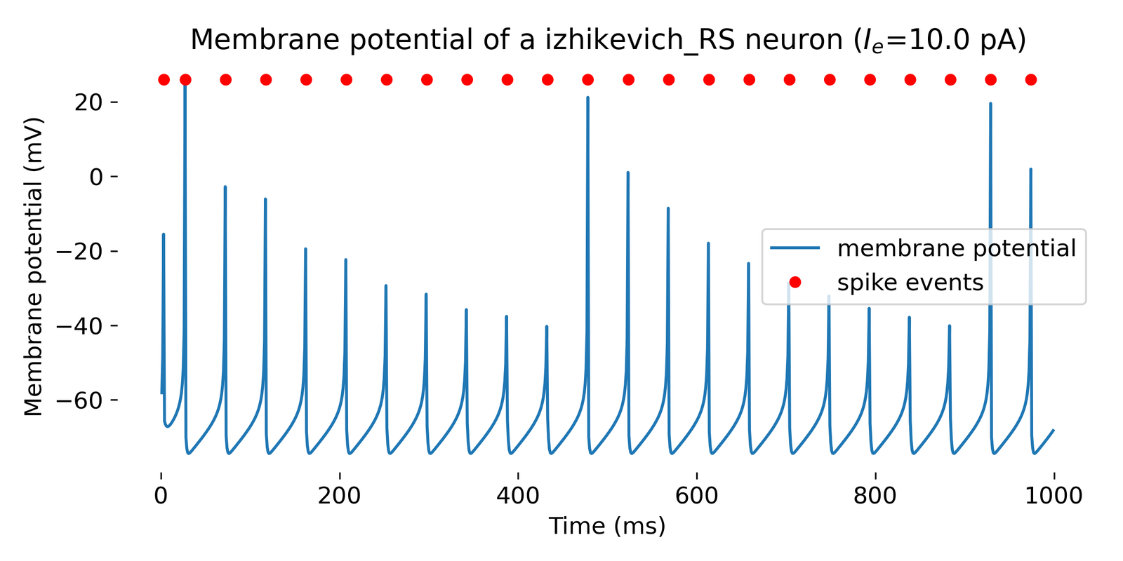
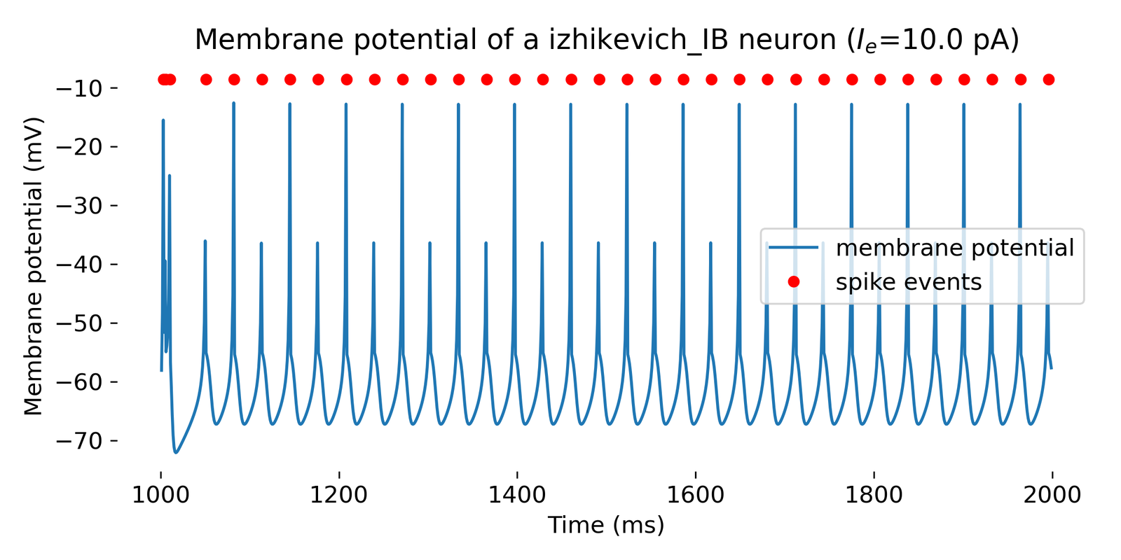
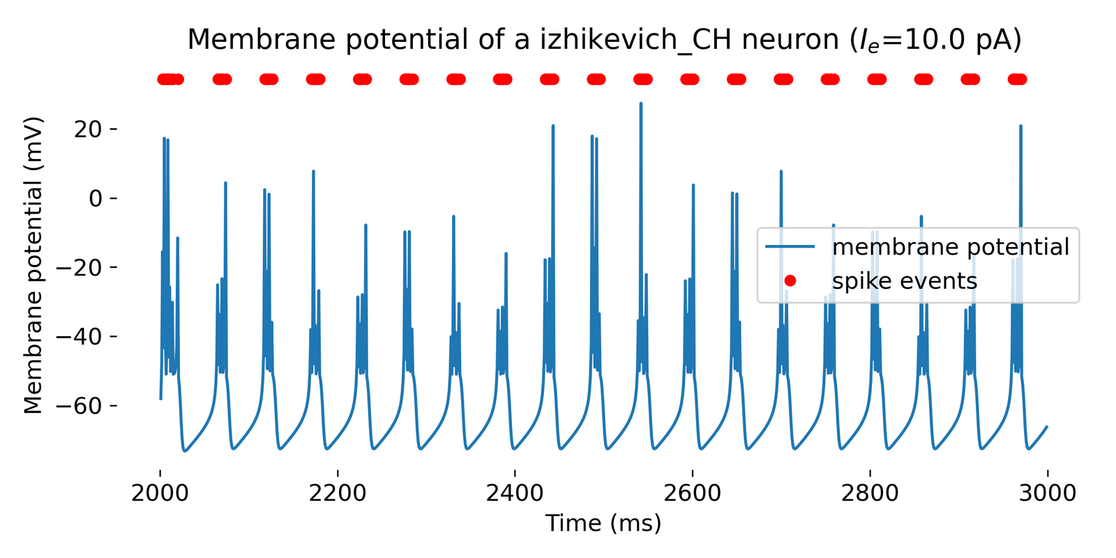
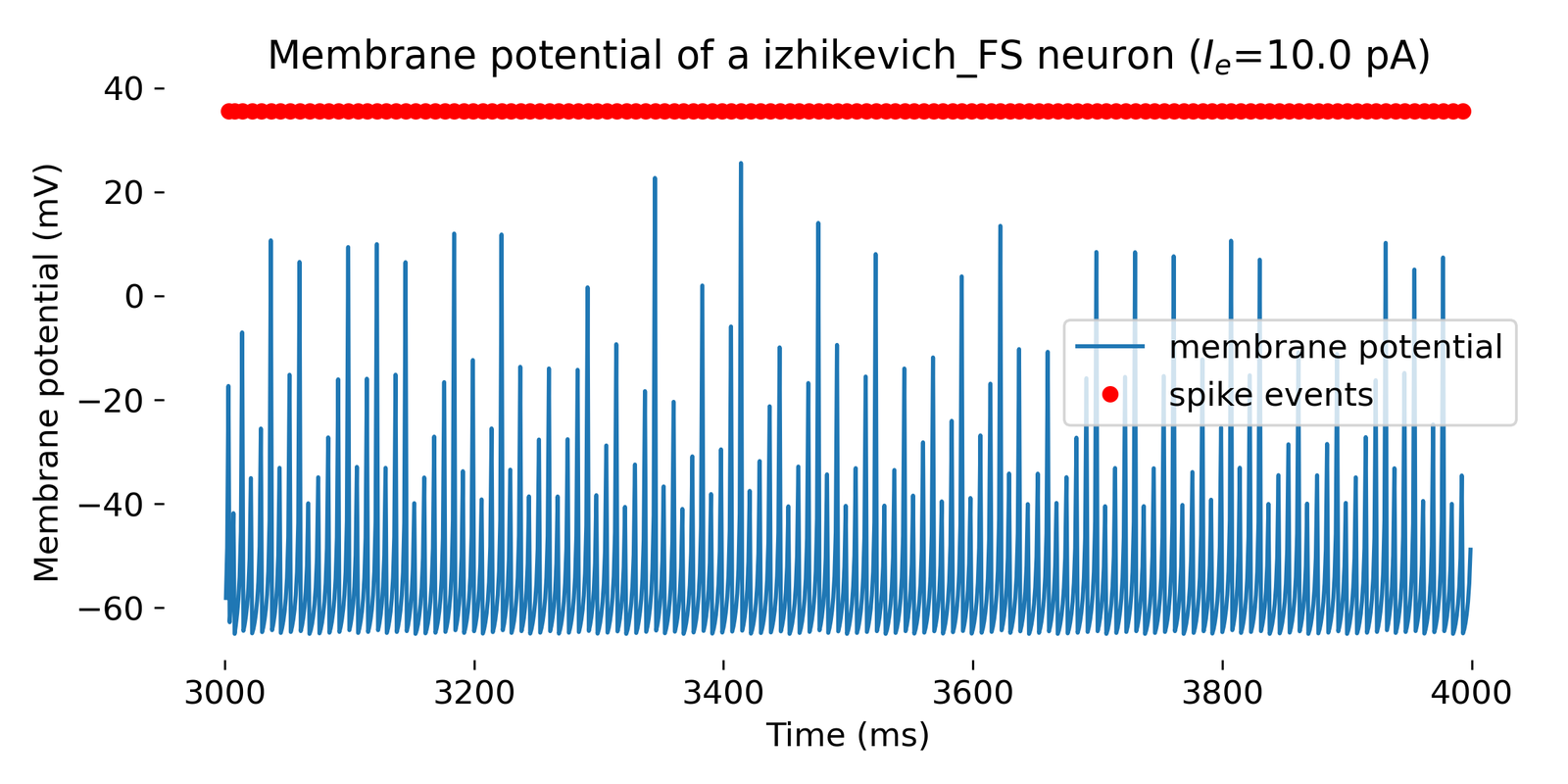
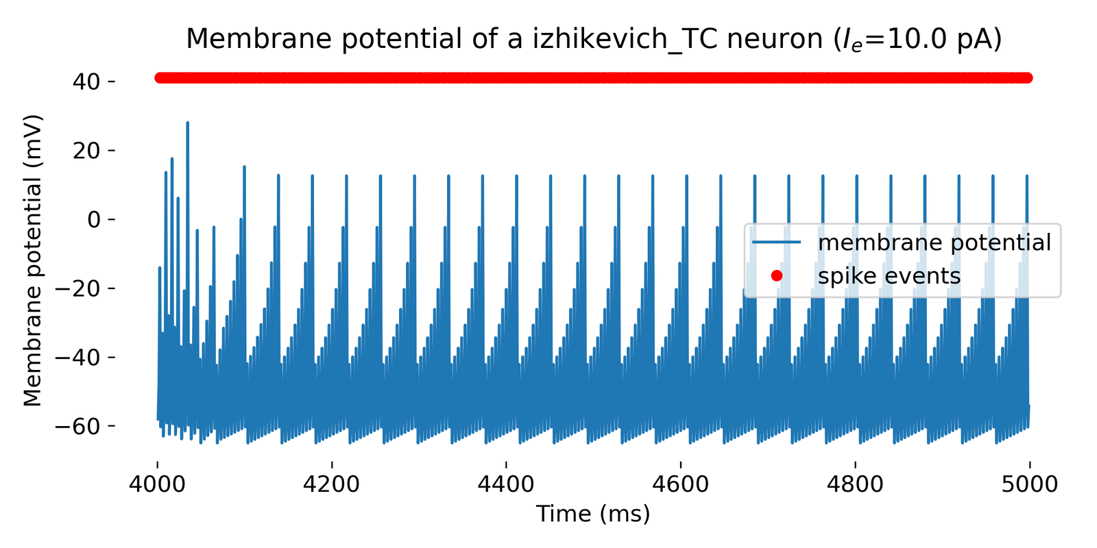
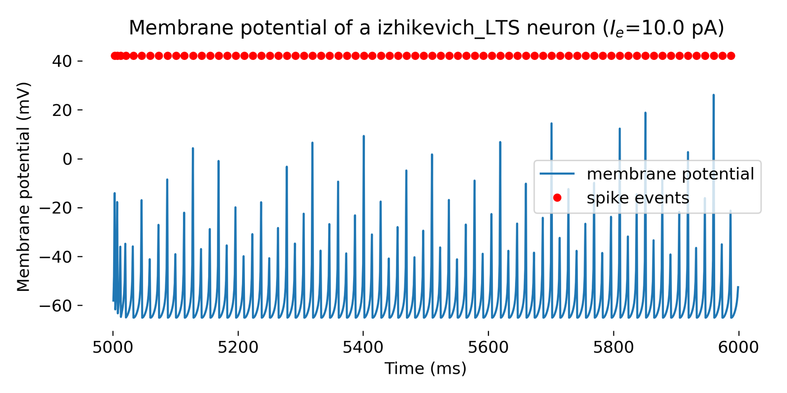
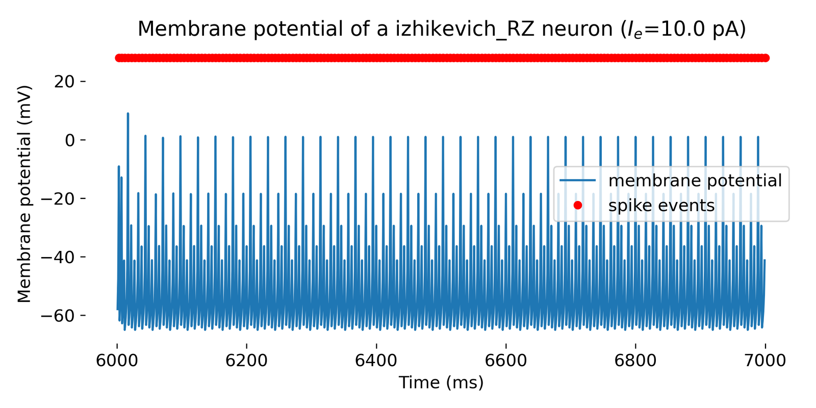Simulated Izhikevich neuron for different parameter sets resulting in different firing patterns, from top to bottom: regular spiking (RS), intrinsically bursting (IB), chattering (CH), fast spiking (FS), thalamic-cortical (TC), low-threshold spiking (LTS), and resonator (RZ). The simulation was run for 1000 ms.

Connecting multiple neurons to a single recording device

In the last example you may have noticed that the time for each simulation was not reset. For each new simulation, the time array starts where the previous simulation ended. This is actually due to a mistake that I made in the simulation. I should have reset the kernel before each simulation in the for loop (which unfortunately would have deleted our individual Izhikevich model copies) or created an individual recording device for each model. However, this brings up an important point in NEST regarding the attachment of a single recording device to multiple neurons. If you connect a single recording device to multiple neurons or neuron populations, the data for each $n$ neuron will be stored in a nested format. Thus, to extract the data in the correct order, you need to sliceꜛ the data array with a step. Here is an exampleꜛ:

# create two neuron nodes:
neuron1 = nest.Create("iaf_psc_alpha")
neuron1.set({"I_e": 340.0})
neuron2 = nest.Create("iaf_psc_alpha")
neuron2.set({"I_e": 370.0})

# create a multimeter node:
multimeter = nest.Create("multimeter")
multimeter.set(record_from=["V_m"])
spikerecorder = nest.Create("spike_recorder")

# connect all nodes:
nest.Connect(multimeter, neuron1)
nest.Connect(multimeter, neuron2)

nest.Simulate(1000.0)

To retrieve the data from the multimeter in the correct order you need to correctly slice the data array:

mm   = multimeter.get()
Vms1 = mm["events"]["V_m"][::2] # start at index 0: till the end: each second entry
ts1  = mm["events"]["times"][::2]

Vms2 = mm["events"]["V_m"][1::2] # start at index 1: till the end: each second entry
ts2  = mm["events"]["times"][1::2]

plt.figure(1)
plt.plot(ts1, Vms1)
plt.plot(ts2, Vms2)

Alternative single neuron simulators

While we use NEST to study the behavior of single neurons throughout this tutorial, NEST is primarily designed to simulate large-scale networks of spiking neurons. There are other simulators that are more suitable for single neuron simulations, such as Brian2ꜛ. Brian2 is a simulator for spiking neural networks written in Python that is designed to be easy to use and highly flexible. It is particularly well-suited for single neuron simulations and small networks.

Conclusion

NEST is a robust and versatile simulator designed for large-scale simulations of spiking neural networks. In this tutorial, we have learned the fundamental aspects of using NEST by modeling and simulating the behavior of single neurons. By starting with the installation and setup of NEST, we progressed through the creation and manipulation of individual neuron models, demonstrated how to connect neurons with recording devices, and explored various stimulation paradigms.

Understanding the behavior of single neurons is crucial as it forms the building block for more complex network simulations. With the skills and knowledge gained from this tutorial, you are now ready to explore and create intricate neural network models. In my next posts, we will learn how to extend these concepts into multi-neuron networks and large-scale simulations, further uncovering the potential of NEST.

The complete code used in this blog post is available in this Github repositoryꜛ. Feel free to modify and expand upon it, and share your insights.

References and useful links

• Gewaltig, M.-O., & Diesmann, M., NEST (NEural Simulation Tool), 2007 Scholarpedia, 2(4), 1430, doi: 10.4249/scholarpedia.1430ꜛ
• Documentation of the NEST simulatorꜛ
• PyNEST API listingꜛ
• List of all supported neuron and synapse models in NESTꜛ
• NEST Tutorial “Part 1: Neurons and simple neural networks”ꜛ
• NEST tutorial “One neuron example”ꜛ
• NEST tutorial “One neuron with noise”ꜛ
• NEST tutorial “Two neuron example”ꜛ