Spike-timing-dependent plasticity (STDP)

February 12, 2026 26 minute read see also comments

Another frequently used term in computational neuroscience is spike-timing-dependent plasticity (STDP). STDP is a form of synaptic plasticity in which the strength of a synaptic connection is modified as a function of the precise temporal relationship between presynaptic and postsynaptic spikes. Rather than depending on averaged firing rates or stimulation frequency alone, STDP operates on the millisecond timescale of individual action potentials.

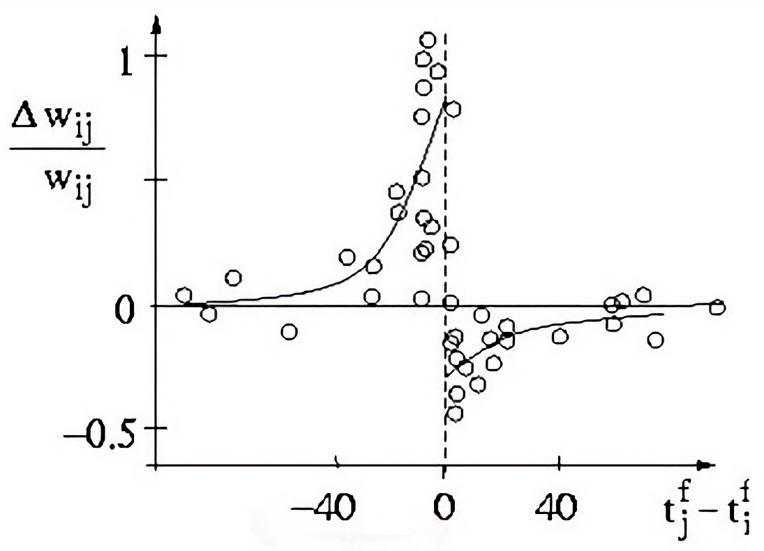
The plot illustrates the relationship between the change in synaptic weight ($\Delta w_{ij} / w_{ij}$) and the time difference ($t_j^f - t_i^f$) between the firing of the presynaptic neuron ($t_i^f$) and the postsynaptic neuron ($t_j^f$; $f$ denotes the spike index). For positive time differences, the synaptic weight increases, leading to long-term potentiation (LTP). For negative time differences, the synaptic weight decreases, resulting in long-term depression (LTD). The magnitude of the change in synaptic weight is determined by the time constants $\tau_+$ and $\tau_-$ for potentiation and depression, respectively (see explanation below). Source: scholarpedia.orgꜛ (modified; after Bi and Poo (1998)ꜛ)

Spike-timing-dependent plasticity

Spike-timing-dependent plasticity is a specific form of synaptic plasticity that depends on the precise timing of spikes (action potentials) between pre- and postsynaptic neurons. The change in synaptic strength is directly influenced by the relative timing of these spikes.

What is a synapse?

Before we continue, it is important to clarify what we mean by a “synapse” when we use this term.

First of all, a synapse is not a virtual construct or purely theoretical connection. It is a real anatomical structure that can be identified under the microscope. At the same time, in computational models it is represented in a strongly simplified and abstract form. It is important to clearly distinguish these two levels.

Anatomical synapse

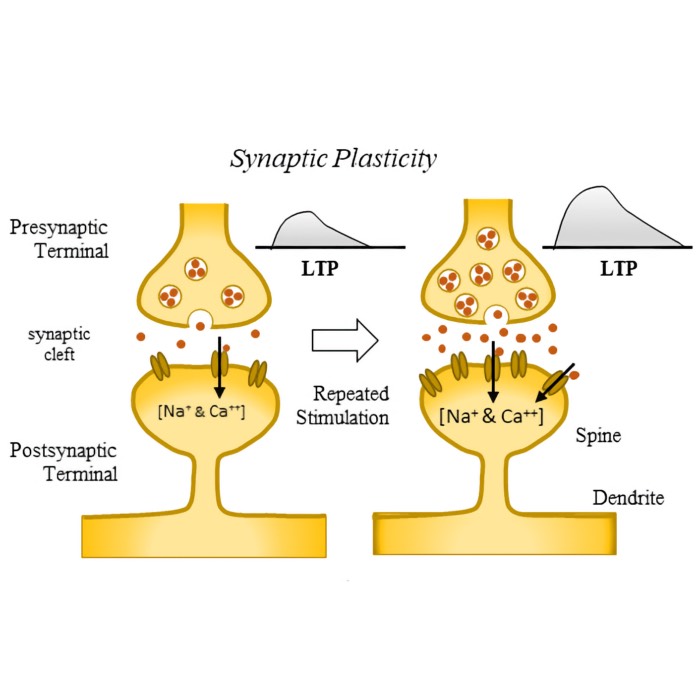
In biological tissue, a synapse is a specialized contact structure between two neurons. It consists of three main components:

a presynaptic terminal containing synaptic vesicles filled with neurotransmitter,
a narrow synaptic cleft (about 20–40 nm wide),
a postsynaptic membrane equipped with specific receptors and a dense protein scaffold.

Schematic representation of an anatomical synapse: The presynaptic terminal contains synaptic vesicles filled with neurotransmitter, which are released into the synaptic cleft upon arrival of an action potential. The postsynaptic membrane contains receptors that bind the neurotransmitter and initiate a postsynaptic response. Source: Wikimedia Commonsꜛ (license: CC BY-SA 4.0)

This tripartite structure (not to be confused with the tripartite synapse, see below) is clearly visible, e.g., in electron microscopy and is, therefore, a real physical entity and not just a conceptual placeholder. However, please also note, that

Functionally, a synapse is the site where:

an action potential arrives presynaptically,
neurotransmitter is released,
postsynaptic receptors are activated,
and a postsynaptic current or conductance change is generated.

It is the elementary unit of signal transmission between neurons.

Synapses in computational models

In theoretical and computational neuroscience, a synapse is abstracted to:

a directed connection from neuron $j$ to neuron $i$,
a single scalar weight $w_{ij}$,
optionally additional internal state variables such as eligibility traces.

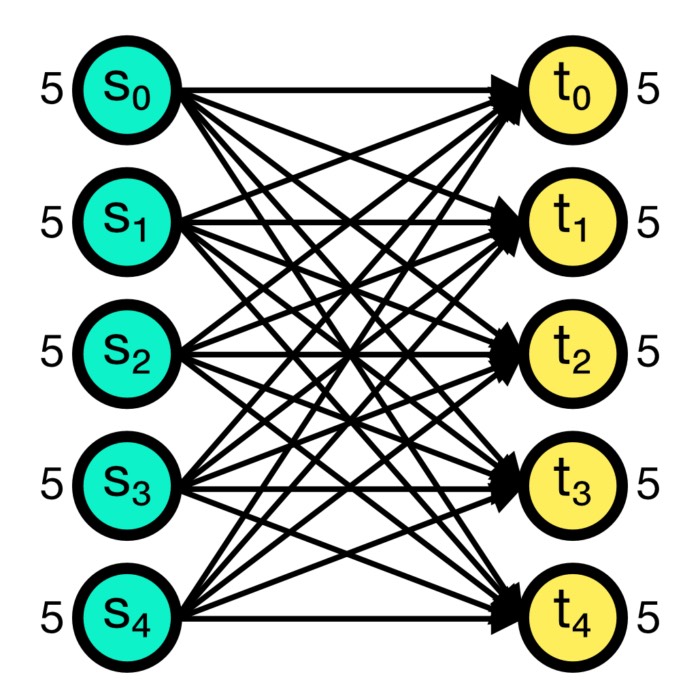
Schematic representation of a synapse in computational models: Presynaptic neurons $x_i$ project to a postsynaptic neuron $y$ with corresponding synaptic weights $w_i$. The postsynaptic activity $y$ is the sum of the products of presynaptic activities and synaptic weights.

This weight summarizes the effective coupling strength between two neurons. It compresses a highly complex molecular and structural system into a single number.

In reality, a synapse involves:

probabilistic vesicle release,
receptor kinetics,
nonlinear dynamics,
structural plasticity,
and many interacting proteins.

The model does not reproduce this complexity. It captures only the effective transmission strength and its modification.

The anatomical synapse described above is referred to as a “chemical synapse”. There are also “electrical synapses” (gap junctions) that allow direct electrical coupling between neurons, but they are not the focus of this discussion. However, we discussed them already in our post on gap junctions.

The tripartite synapse

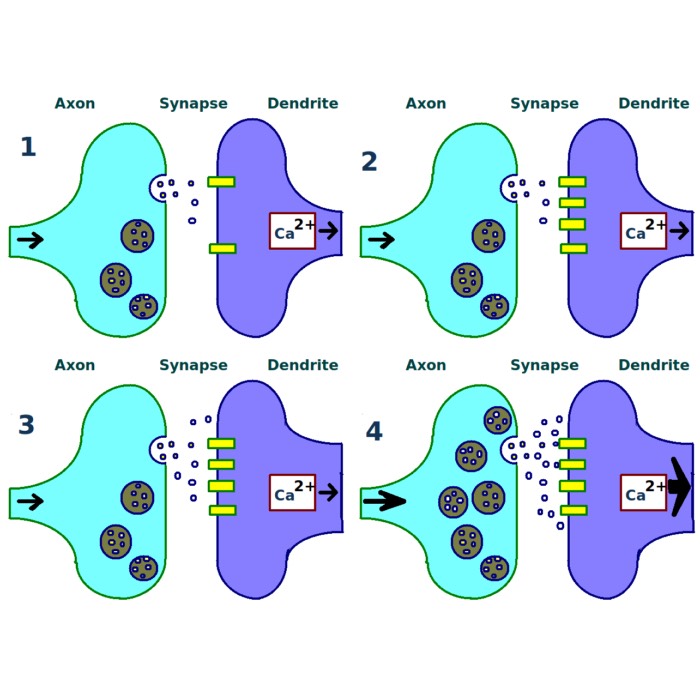
The anatomical picture described above was substantially refined when it became clear that astrocytes, a type of glial cell, actively participate in synaptic signaling. Araque et al. (1999)ꜛ demonstrated that astrocytes are not merely passive support cells, but can detect synaptic activity, respond with intracellular calcium elevations, and in turn modulate synaptic transmission.

Schematic representation of glutamate reuptake at an excitatory synapse. The presynaptic terminal releases glutamate, which binds to postsynaptic receptors and is subsequently cleared by astrocytic transporters (EAAT2/GLT1). This functional integration of presynaptic terminal, postsynaptic membrane, and surrounding astrocytic processes is referred to as the tripartite synapse. Source: Wikimedia Commonsꜛ (license: CC BY-SA 4.0)

Astrocytic processes closely enwrap many excitatory synapses. They express neurotransmitter receptors, particularly for glutamate, allowing them to sense synaptic release. Upon activation, astrocytes can regulate extracellular neurotransmitter concentrations through uptake mechanisms, thereby shaping synaptic efficacy and preventing excitotoxicity. Moreover, astrocytes have been reported to release so-called gliotransmitters such as glutamate, ATP, or D-serine, although the physiological relevance and mechanisms of such release remain an active area of debate.

This led to the concept of the tripartite synapse, consisting of:

the presynaptic terminal,
the postsynaptic membrane,
and the surrounding astrocytic process.

In this framework, synaptic transmission is no longer viewed as a purely neuronal two-element interaction. Instead, it is embedded in a local neuron–glia microcircuit in which astrocytes dynamically regulate information flow and plasticity. While many computational models treat the synapse as a two-body interaction between pre- and postsynaptic neurons, the biological reality is more complex and includes glial modulation as an additional regulatory layer, which is an active area of ongoing research.

One more subtle point

Between two neurons, there can be multiple anatomical synapses. In most network models, these are represented as a single effective connection with one weight parameter.

Thus, when we speak of “a synapse” in numerical simulations, we refer to a simplified mathematical representation of a real, anatomically defined contact structure.

I think, understanding this distinction prevents conceptual confusion when moving between biology and mathematical modeling.

In STDP, the direction and magnitude of synaptic changes depend on whether the presynaptic spike precedes the postsynaptic spike or vice versa. Empirically, STDP exhibits the following characteristic behavior:

If a presynaptic neuron fires shortly before a postsynaptic neuron, typically within a temporal window of 10 to 20 ms, the synapse is strengthened. This corresponds to long-term potentiation (LTP).
If the presynaptic neuron fires shortly after the postsynaptic neuron, the synapse is weakened. This corresponds to long-term depression (LTD).

In contrast to classical experimental protocols for long-term potentiation and long-term depression, which are typically defined and induced using sustained patterns of stimulation such as prolonged high-frequency or low-frequency input, spike-timing-dependent plasticity emphasizes the fine temporal structure of neuronal activity. Rather than averaging activity over extended time windows, STDP operates on the millisecond timescale of individual action potentials and explicitly encodes the relative order of presynaptic and postsynaptic spikes.

This focus on spike timing introduces a causal interpretation of synaptic modification. Synapses are strengthened when presynaptic activity reliably precedes postsynaptic firing, indicating a predictive contribution to postsynaptic activation, and weakened when this temporal order is reversed. In this sense, STDP provides a temporally precise and biologically plausible description of how synaptic changes can arise directly from ongoing spiking activity in neural circuits, without requiring artificial stimulation protocols.

Although STDP and classical LTP and LTD are often discussed as separate forms of plasticity, they should not be regarded as distinct mechanisms. Instead, STDP captures a specific temporal organization of synaptic modification that can give rise to LTP-like or LTD-like changes when considered over longer timescales. Depending on the statistics of spike timing, repeated pre-before-post pairings lead to net potentiation, while repeated post-before-pre pairings lead to net depression.

At the mechanistic level, STDP and classical LTP and LTD share common intracellular substrates. Both involve NMDA receptor activation, calcium influx, and downstream signaling cascades that ultimately modify synaptic efficacy. The primary distinction between these descriptions therefore does not lie in the underlying biological machinery, but in the temporal resolution at which synaptic changes are formulated and analyzed. STDP provides a spike-based, temporally resolved framework that complements and refines the rate- and protocol-based descriptions traditionally used to characterize LTP and LTD.

Mathematical formulation of STDP

STDP can be considered a form of Hebbian learning that refines the concept by incorporating precise spike timing.

Let us consider a simple mathematical model for STDP. We can describe the change in synaptic weight, $\Delta w_{ij}$ between two neurons $i$ and $j$ as a function of the time difference between their spikes ($t_j^n - t_i^f$), where $f=1, 2,3, \ldots$ counts the presynaptic spikes spikes of neuron $i$ (presynaptic), $n=1, 2,3, \ldots$ counts the postsynaptic spikes of neuron $j$ (postsynaptic). The total change in synaptic weight can be expressed as follows:

\[\begin{align} \Delta w_{ij} = \sum_{f=1}^{N_i} \sum_{n=1}^{N_j} W(t_j^n - t_i^f) \end{align}\]

where $W(t_j^n - t_i^f)$ denotes the chosen STDP function, also called learning window. The STDP function $W(t_j^n - t_i^f)$ typically follows an exponential decay function, where the change in synaptic weight depends on the time difference between the spikes. A commonly used form of the learning window is an asymmetric exponential function:

\[\begin{equation} W(t_j^n - t_i^f) = \begin{cases} A_+ \exp\!\left(-\dfrac{t_j^n - t_i^f}{\tau_+}\right), & \text{if } t_j^n - t_i^f > 0 \\ -A_- \exp\!\left(\frac{t_j^n - t_i^f}{\tau_-}\right), & \text{if } t_j^n - t_i^f < 0 \end{cases} \end{equation}\label{eq:stdp}\]

Here, $A_+$ and $A_-$ are scaling factors, while $\tau_+$ and $\tau_-$ are time constants for potentiation and depression, respectively. They are typically in the order of 10 ms. Key features of this model include:

when the time difference is positive ($t_j^n - t_i^f > 0$), i.e., that presynaptic neuron fired before the postsynaptic neuron, it typically leads to long-term potentiation (LTP) where the synaptic strength increases.
when the time difference is negative ($t_j^n - t_i^f < 0$), indicating that the postsynaptic neuron fired before the presynaptic neuron, it generally results in long-term depression (LTD), where the synaptic strength decreases.

Graphical representation of STDP

Let’s plot the learning window function Eq. $\eqref{eq:stdp}$ to further understand these relationships:

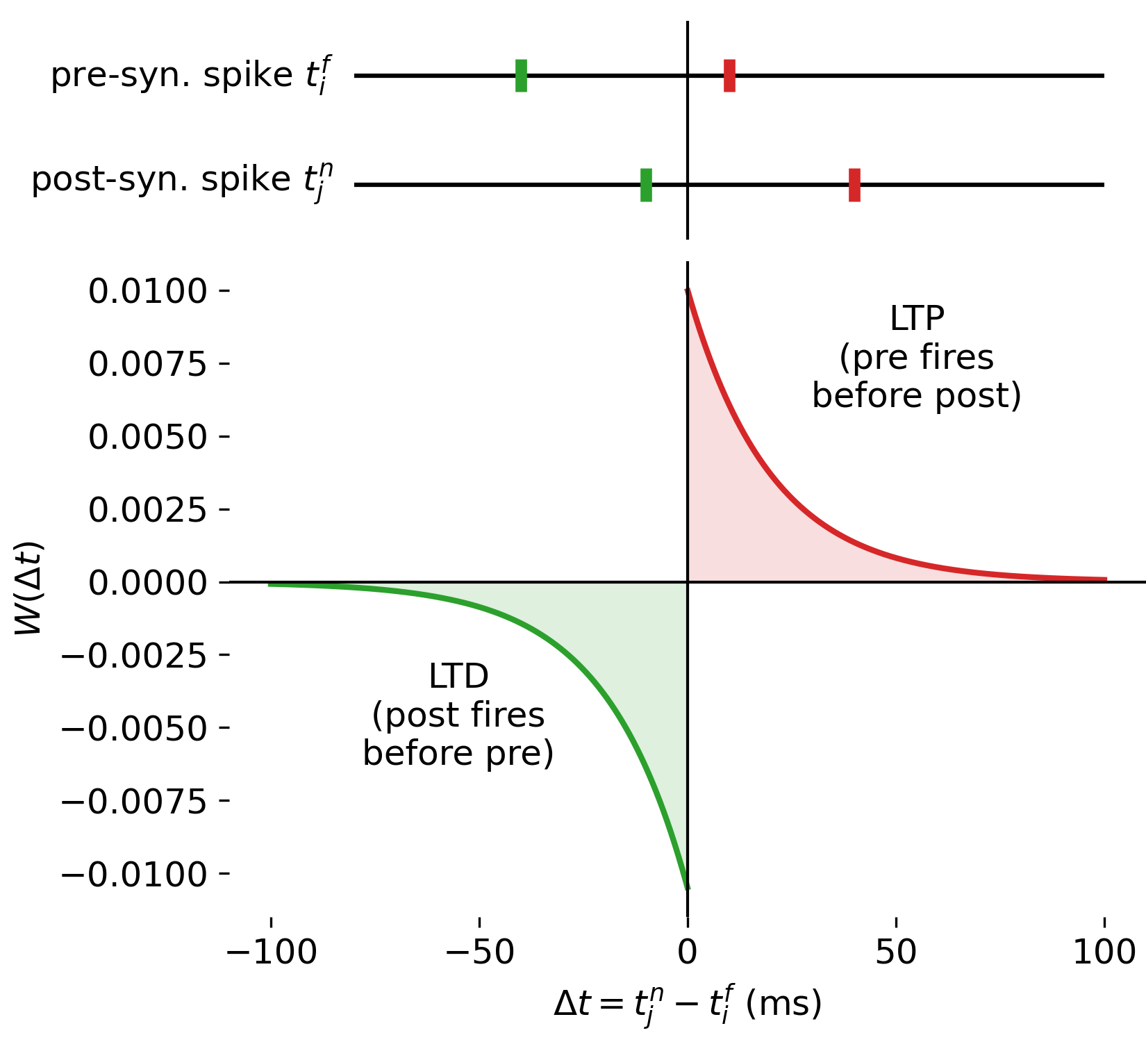
STDP learning window $W(\Delta t)$ as a function of the relative spike timing $\Delta t = t_j^n - t_i^f$. The lower panel shows the change in synaptic weight induced by a single pre–post spike pair, with potentiation (LTP) for $\Delta t > 0$ (i.e., $t_i^f < t_j^n$) and depression (LTD) for $\Delta t < 0$ (i.e., $t_j^n < t_i^f$). The upper panel provides a schematic illustration of individual pre–post spike pairs corresponding to specific points on the learning window. The Python code used to generate this figure is available in the GitHub repository mentioned at the end of the post.

Shown here is STDP for a single, directed synapse, connecting a presynaptic neuron $i$ to a postsynaptic neuron $j$, with synaptic weight $w_{ij}$.

The lower panel shows the STDP learning window $W(\Delta t)$ as a function of the relative spike timing

\[\Delta t = t_j^n - t_i^f.\]

Again, $t_i^f$ denotes the spike time of the presynaptic neuron and $t_j^n$ the spike time of the postsynaptic neuron. The vertical axis represents the change in synaptic weight induced by a single pre–post spike pair.

The learning window is asymmetric around $\Delta t = 0$, and as described before, two distinct regimes can be identified based on the sign of $\Delta t$:

For $\Delta t > 0$, the presynaptic neuron fires before the postsynaptic neuron (“pre fires before post”), i.e., $t_i^f < t_j^n$. This is illustrated in the upper panel (right side, red marks), where the spike of the presynaptic neuron is closer to the $\Delta t = 0$ line, indicating its earlier firing, followed by the later spike of the postsynaptic neuron at a larger positive $\Delta t$. In this case, the spiking of the presynaptic neuron can be interpreted as contributing causally to the firing of the postsynaptic neuron. The synapse is therefore potentiated and the weight change is positive, corresponding to long-term potentiation (LTP).
For $\Delta t < 0$, the postsynaptic neuron fires before the presynaptic neuron (“post fires before pre”), i.e., $t_j^n < t_i^f$. This is illustrated in the upper panel (left side, green marks), where the spike of the postsynaptic neuron is closer to the $\Delta t = 0$ line, indicating its earlier firing, followed by the later spike of the presynaptic neuron at a larger negative $\Delta t$. In this case, the presynaptic spike is less likely to have contributed to the postsynaptic firing, and the synapse is depressed, leading to a negative weight change corresponding to long-term depression (LTD).

The exponential decay of both branches reflects the decreasing influence of spike pairs as their temporal separation increases. Spike pairs with large absolute time differences contribute only weakly to synaptic modification.

The color coding (red and green) emphasizes the functional distinction between LTD and LTP regimes (and not the neuron identity).

Together, the two panels demonstrate how STDP maps the relative timing of individual pre- and postsynaptic spikes onto systematic synaptic weakening or strengthening. Absolute spike times are irrelevant for the learning rule. Only the temporal order and separation of spikes determine the direction and magnitude of synaptic change, with larger temporal proximity leading to stronger modifications. This illustrates the core principle of STDP as a local, spike-based learning mechanism that encodes causal relationships between neuronal activity patterns at the level of individual synapses.

Incorporating STDP in neuron models

To incorporate STDP in a neuron model, we need to make the following assumptions. Each presynaptic spike arrival leaves a trace variable $x_i(t)$ that is updated by an amount $a_+(x_i)$, and, similarly, each postsynaptic spike arrival leaves a trace variable $y_j(t)$ that is updated by an amount $a_-(y_j)$. Both traces exponentially decay with time constants $\tau_+$ and $\tau_-$ in absence of spikes:

\[\begin{align} \tau_+ \frac{dx_i}{dt} &= -x_i + a_+(x_i)\sum_f \delta(t - t_i^f), \\ \tau_- \frac{dy_j}{dt} &= -y_j + a_-(y_j)\sum_n \delta(t - t_j^n) \end{align}\]

where:

$x_i(t)$ is a trace variable for the presynaptic spikes
$y_j(t)$ is a trace variable for the postsynaptic spikes
$\tau_+$ and $\tau_-$ are the time constants for the trace variables.
$a_+(x_i)$ and $a_-(y_j)$ are functions that describe how the trace variables are updated upon the occurrence of spikes.
$w_{ij}$ is the synaptic weight from presynaptic neuron $i$ to postsynaptic neuron $j$

In the simplest and most commonly used case, $a_+(x_i)$ and $a_-(y_j)$ are constants, so that each spike produces a fixed additive increment of the corresponding trace. More general choices allow state-dependent or saturating trace updates, which can be used to model nonlinear effects without changing the overall structure of the STDP rule.

The synaptic weight change according:

\[\begin{equation}\begin{aligned} \frac{dw_{ij}}{dt} = \quad &A_+(w_{ij})\, x_i(t)\sum_n \delta(t - t_j^n) \\ -&A_-(w_{ij})\, y_j(t)\sum_f \delta(t - t_i^f) \end{aligned}\end{equation}\]

The synaptic weight $w_{ij}$ changes based on the trace variables and the occurrence of spikes. The first term, $A_+(w_{ij}) x_i(t) \sum_n \delta(t - t_j^n)$, represents potentiation and depends on the presynaptic trace variable and the occurrence of postsynaptic spikes. The second term, $A_-(w_{ij}) y_j(t) \sum_f \delta(t - t_i^f)$, represents depression and depends on the postsynaptic trace variable and the occurrence of presynaptic spikes.

Python example

To illustrate how to implement STDP in a simple neuron model, this time we use the brian2ꜛ simulator, which is a popular tool for simulating spiking neural networks. The code below defines a simple (postsynaptic) leaky integrate-and-fire neuron receiving input from a population of 1000 Poisson spike generators, with STDP implemented on the synapses. The parameters are chosen to be in a reasonable range for this type of model. The synaptic weights are constrained to be between 0 and a maximum value gmax. We also set up monitors to record the synaptic weights over time and the presynaptic spike times. The code is available in the GitHub repository mentioned at the end of the post. It is originally based on the example provided in the brian2 documentation: Spike-timing-dependent plasticity (STDP)ꜛ:

import os
from pdb import run
from turtle import clear
import brian2 as b2
from brian2 import ms, mV, nS, Hz, second
import matplotlib.pyplot as plt

# set global properties for all plots:
plt.rcParams.update({'font.size': 12})
plt.rcParams["axes.spines.top"]    = False
plt.rcParams["axes.spines.bottom"] = False
plt.rcParams["axes.spines.left"]   = False
plt.rcParams["axes.spines.right"]  = False

# define parameters:
N = 1000            # number of presynaptic neurons
taum = 10*ms        # membrane time constant
taupre = 20*ms      # STDP time constant for presynaptic trace
taupost = taupre    # STDP time constant for postsynaptic trace (often set equal to taupre)
Ee = 0*mV           # excitatory reversal potential
vt = -54*mV         # spike threshold
vr = -60*mV         # reset potential
El = -74*mV         # leak reversal potential
taue = 5*ms         # excitatory synaptic time constant
F = 15*Hz           # firing rate of Poisson input
gmax = .01          # maximum synaptic weight
dApre = .01         # increment applied to the presynaptic eligibility trace Apre on each presynaptic spike (sets the scale of potentiation via Apre)
dApost = -dApre * taupre / taupost * 1.05  # increment applied to the postsynaptic eligibility trace Apost on each postsynaptic spike (negative; slightly stronger magnitude as a stabilizing heuristic)
dApost *= gmax      # scale trace increments to the same order of magnitude as w (since Apre/Apost are added directly to w)
dApre *= gmax       # same scaling for Apre

RESULTS_PATH = "figures"
os.makedirs(RESULTS_PATH, exist_ok=True)

# define the brian2 model with STDP synapses
eqs_neurons = '''
dv/dt = (ge * (Ee-v) + El - v) / taum : volt
dge/dt = -ge / taue : 1
'''

poisson_input = b2.PoissonGroup(N, rates=F)
neurons = b2.NeuronGroup(1, eqs_neurons, threshold='v>vt', reset='v = vr',
                      method='euler')

S = b2.Synapses(poisson_input, neurons,
             '''w : 1
                dApre/dt = -Apre / taupre : 1 (event-driven)
                dApost/dt = -Apost / taupost : 1 (event-driven)''',
             on_pre='''ge += w
                    Apre += dApre
                    w = clip(w + Apost, 0, gmax)''',
             on_post='''Apost += dApost
                     w = clip(w + Apre, 0, gmax)''')
S.connect() # all-to-one connectivity from the Poisson input to the single postsynaptic neuron
S.w = 'rand() * gmax' # random initialization of weights between 0 and gmax
mon = b2.StateMonitor(S, 'w', record=[0, 1]) # record the weights of two example synapses to see how they evolve over time

# run the simulation:
b2.run(100*b2.second, report='text')

# plots:
plt.figure(figsize=(5, 8))
plt.subplot(3, 1, 1)
plt.plot(S.w / gmax, '.', c='mediumaquamarine', markersize=4)
plt.ylabel('w/gmax')
plt.xlabel('synapse index')
plt.title('STDP: weights after simulation')

plt.subplot(3, 1, 2)
plt.hist(S.w / gmax, 20, color='mediumaquamarine')
plt.xlabel('w/gmax')
plt.title('STDP: weight distribution')

plt.subplot(3, 1, 3)
plt.plot(mon.t/b2.second, mon.w[0]/gmax, label='Synapse 0')
plt.plot(mon.t/b2.second, mon.w[1]/gmax, label='Synapse 1')
plt.xlabel('t [s]')
plt.ylabel('w/gmax')
plt.ylim(0.0,1.1)
plt.legend()
plt.title('STDP: example synapses vary over time')

plt.tight_layout()
plt.savefig(os.path.join(RESULTS_PATH, "stdp_example_weights.png"), dpi=300)
plt.close()

In order to compare the sme neuron model with and without STDP, you can simply define a second set of synapses without the STDP rule (i.e., with fixed weights) and run the simulation again:

# weights that do not change over time:
S2 = b2.Synapses(
    poisson_input, neurons,
    model='w : 1',
    on_pre='ge += w')
S2.connect()

This allows you to directly observe the effects of STDP on synaptic weight evolution and neural activity patterns.

After running this simulation, we end up with two plots:

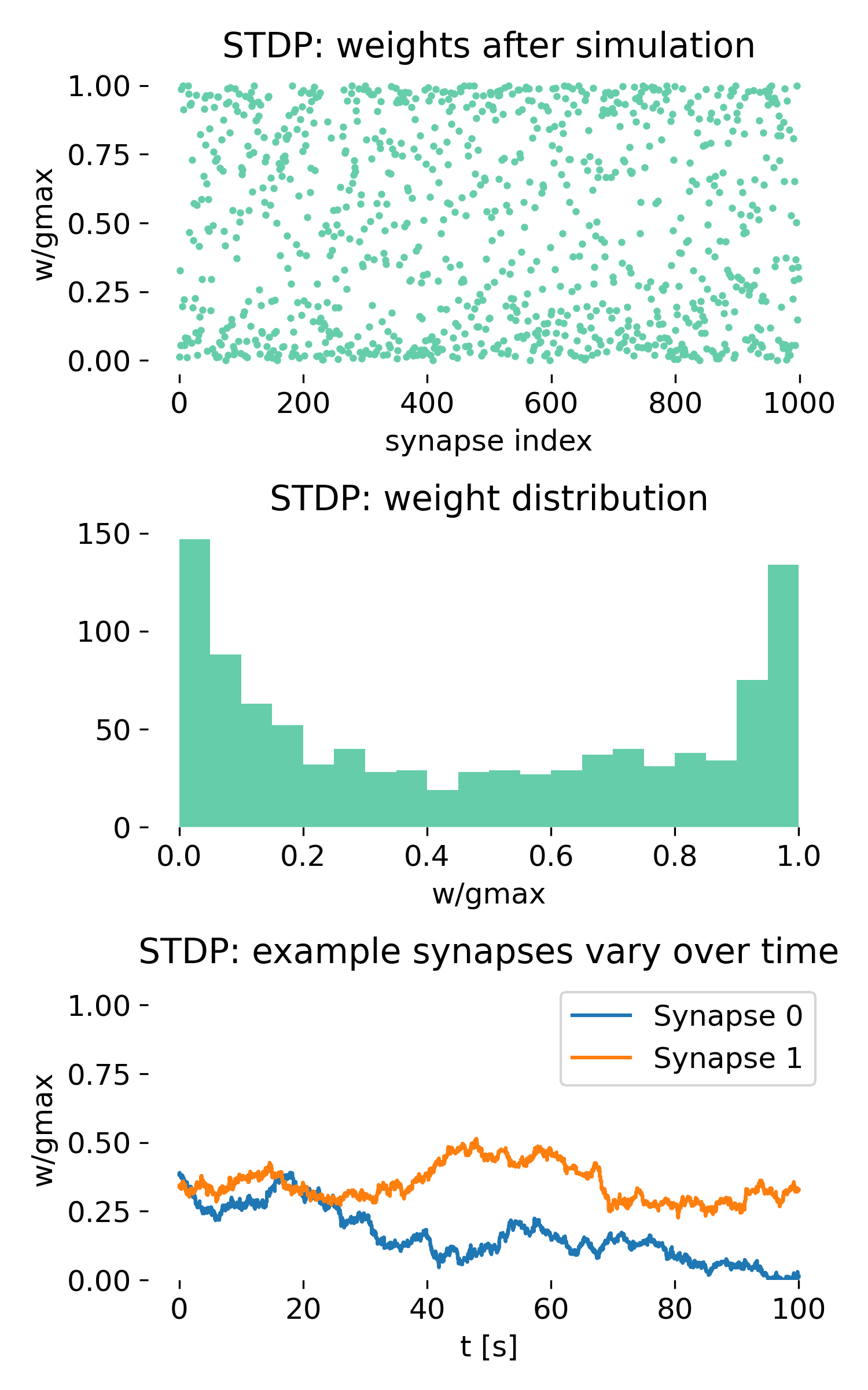
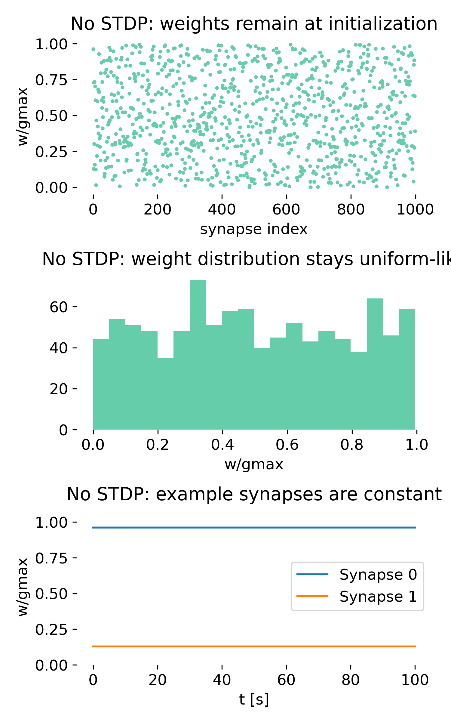
Synaptic weight dynamics with and without spike-timing-dependent plasticity. Left: STDP-enabled network. Synaptic weights differentiate over time and converge toward a bimodal distribution. Right: Control simulation without STDP. Synaptic weights remain at their initial random values and show no dynamical reorganization. Top panels show the final synaptic weights, middle panels show the distribution of synaptic weights, and bottom panels show the time course of two example synapses.

Shown are the results of the simulation with STDP (left) and without STDP (right). For each, three panels are shown, which show from top to bottom:

The synaptic weights after the simulation as a function of synapse index.
The histogram of synaptic weights.
The time course of two example synapses.

Importantly, the upper panel in each column is not a spike raster. It does not contain temporal information. Instead, it shows a single point per synapse representing the final synaptic weight after learning. The x-axis enumerates synapses, while the y-axis shows the normalized weight $w/g_{\max}$.

Network with STDP

Let’s first discuss the results with STDP (left column).

Final weights across synapses (upper panel)

In the STDP condition, the upper panel immediately reveals a strong differentiation of synaptic weights. Although all presynaptic neurons fire statistically identical Poisson spike trains, the synapses do not remain equivalent. Instead, we observe:

a strong spread of final weights,
many synapses clustered near 0,
many synapses clustered near $g_{\max}$,
relatively few synapses in the intermediate regime,
no spatial structure (synapse index is meaningless).

There is no spatial structure along the synapse index, i.e., the structure exists purely in the distribution of weights, not in their arrangement.

This is already a nontrivial result. The network began with homogeneous random weights and statistically identical inputs. Nevertheless, STDP has broken this symmetry and generated synaptic differentiation.

This plot answers exactly one question: What do the synaptic weights look like across all synapses after learning?

The answer is clear: they no longer reflect their random initialization. Instead, they exhibit a pronounced polarization toward the boundaries of the allowed range. Most synapses have either weakened substantially or strengthened close to the maximum value, while comparatively few remain in an intermediate state.

This is a hallmark of STDP dynamics under unstructured input. The learning rule amplifies small random differences in spike timing, leading to a competitive process that pushes synapses toward extreme values. The result is a bimodal distribution of synaptic weights, with many synapses effectively “winning” (potentiated) and many “losing” (depressed), while few remain in an intermediate state.

Weight distribution (middle panel)

The histogram in the middle panel makes this effect quantitative. The distribution is clearly bimodal:

one peak close to 0,
one peak close to $g_{\max}$,
a depletion of weights in the middle.

This is the classical signature of additive, pair-based STDP under unstructured input. Synapses that, by chance, participate slightly more often in causal pre-before-post pairings are reinforced. Synapses that experience slightly more post-before-pre pairings are weakened. Because the learning rule is additive and asymmetric, these small differences are amplified over time.

The process resembles unsupervised synaptic competition. It is not overfitting, nor is it a numerical artifact. It is the expected behavior of this learning rule in the absence of additional stabilizing mechanisms.

Time course of individual synapses (lower panel)

The lower panel shows the evolution of two example synapses. Both exhibit stochastic fluctuations, yet their trajectories display a clear long-term drift. One synapse gradually decreases toward zero, the other drifts upward.

This illustrates several fundamental properties of STDP:

The dynamics are stochastic.
The process is path-dependent.
Early random fluctuations can bias long-term outcomes.
The system tends toward stable boundary states.

STDP here does not fine-tune weights toward a specific optimum. Instead, it acts as a selective amplification mechanism that pushes synapses toward extreme states.

Why do weights accumulate near 0 and $g_{\max}$?

So, why do the weights accumulate near the boundaries? Why do we see this bimodal distribution instead of a more uniform spread?

The bimodal outcome arises from the structure of the learning rule itself. Formally, the update mechanism in the simulation is:

on presynaptic spikes: $w \leftarrow \mathrm{clip}(w + A_{\text{post}}, 0, g_{\max})$
on postsynaptic spikes: $w \leftarrow \mathrm{clip}(w + A_{\text{pre}}, 0, g_{\max})$

with positive LTP contributions and slightly stronger LTD contributions.

This is not gradient descent on a global objective. It is a stochastic drift process. For independent Poisson input, causal and anti-causal spike pairings occur with approximately equal probability. However:

LTD is slightly stronger than LTP.
Postsynaptic firing depends on the current synaptic weight.
Weights are clipped at 0 and $g_{\max}$.

As a consequence:

Intermediate weights are unstable.
Small weights tend to drift further downward.
Large weights tend to drift further upward.
The boundaries at 0 and $g_{\max}$ act as stable attractors.

The result is weight binarization. Synapses are pushed into an either-or regime. This phenomenon has long been known in theoretical studies of additive STDP and is often described as bimodal weight dynamics or winner-take-all behavior at the synaptic level.

Biologically, such pure binarization is unrealistic. Real neural systems require additional mechanisms such as weight-dependent plasticity, homeostatic regulation, normalization, or inhibitory competition to prevent saturation. However, for didactic purposes, this simple setup is ideal. It isolates the intrinsic competitive character of STDP.

Control experiment without STDP

Now, let’s turn to the control simulation without STDP (right column). Here, the synaptic weights are fixed and do not change over time. This allows us to isolate the effects of spiking activity alone, without any plasticity.

Final weights (upper panel)

Without plasticity, the final weights are indistinguishable from the initialization. The distribution across synapse indices remains random. No synapse is selected, no differentiation emerges.

Weight distribution (middle panel)

The histogram remains approximately uniform over $[0, g_{\max}]$. Any deviations are due to finite sampling, not dynamics. There is no drift, no bimodality, no boundary accumulation. This means, that the distribution reflects only the initial random assignment of weights, and that spiking activity alone does not modify synaptic strength. The system remains in a static state with no learning or reorganization.

Time course (lower panel)

The trajectories of the example synapses remain perfectly constant. Despite continuous presynaptic spiking, nothing changes. Spiking activity alone does not modify synaptic strength.

This control condition demonstrates a central point:
Activity does not imply plasticity, i.e., the network does not structure itself just because neurons are spiking. Only when spike timing is coupled to weight updates does structural reorganization occur:

with selection of early vs. later inputs,
with structure in the weight distribution, and
with functional differentiation of synapses.

Thus, we can summarize the functional role of STDP in this minimal model as follows: Without STDP, the network is a passive integrator of random inputs. With STDP, it becomes a system that learns temporal causality, or to be more precise, it becomes a system that reinforces temporal correlations and spike order relationships.

What is actually learned?

It is important to evaluate what this model does and does not achieve.

There is:

no structured input,
no task,
no supervision,
no inhibition, and
no explicit competition beyond STDP itself.

Consequently, the network does not learn semantic structure, features, or representations. It does not classify, predict, or encode meaningful patterns.

What it does demonstrate is more fundamental. STDP alone acts as a self-organizing mechanism that breaks symmetry among statistically identical inputs. It induces synaptic competition and produces structured weight distributions even under pure noise.

The comparison between both simulations makes this transparent:

Without STDP: We end up with static random connectivity.
With STDP: We get dynamic differentiation and weight binarization.
With additional regulatory mechanisms: We would potentially get even meaningful learning.

Thus, this minimal model illustrates how a simple, biologically plausible learning rule can generate nontrivial synaptic structure from unstructured activity. It serves as a foundation for understanding more complex learning dynamics in spiking neural networks.

STDP and Hebbian learning rules

STDP can be viewed as a temporally refined form of Hebbian learning. Classical Hebbian plasticity is often summarized as a correlation-based rule in which synaptic strength increases when presynaptic and postsynaptic activity are correlated. In its simplest rate-based form, Hebbian learning can be written as

\[\frac{d w_{ij}}{d t} \propto r_i r_j,\]

where $r_i$ and $r_j$ are the firing rates of the pre and postsynaptic neurons.

STDP extends this principle by resolving correlations at the level of individual spikes rather than averaged firing rates. By distinguishing pre-before-post from post-before-pre spike pairings, STDP introduces a causal asymmetry that is absent in classical Hebbian rules. Synaptic strengthening occurs when presynaptic activity predicts postsynaptic firing, while synaptic weakening occurs when this temporal order is reversed.

In this sense, STDP implements a temporally precise notion of Hebbian causality rather than mere correlation.

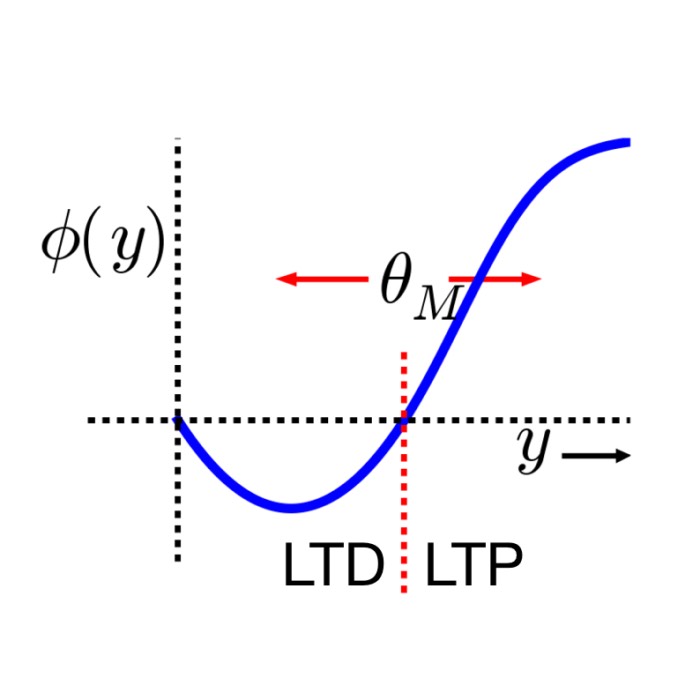
STDP and Bienenstock-Cooper-Munro (BCM) rule

Teh Bienenstock-Cooper-Munro (BCM) rule is a rate-based plasticity model in which synaptic changes depend nonlinearly on postsynaptic activity relative to a sliding threshold. In its classical form, the BCM rule can be written as

\[\frac{d w_{ij}}{d t} = r_i \, \phi(r_j),\]

where $\phi(r_j)$ is a nonlinear function that changes sign at a postsynaptic activity threshold $\theta_M$. This threshold itself depends on the long-term average of postsynaptic activity.

Although STDP is formulated at the spike level, it can give rise to BCM-like behavior when averaged over stochastic spike trains. In particular, when neurons fire as Poisson processes and when extended STDP rules such as triplet-based STDPꜛ are used, the expected synaptic change becomes a nonlinear function of presynaptic and postsynaptic firing rates.

Under these conditions, the average weight change takes the form

\[\langle \Delta w_{ij} \rangle \propto r_i \, r_j (r_j - \theta),\]

where $\theta$ depends on the parameters of the STDP rule and the statistics of postsynaptic firing. This expression mirrors the structure of the BCM rule, with a sliding threshold emerging from spike timing statistics rather than being imposed explicitly.

STDP can therefore be understood as a spike-based mechanism from which rate-based learning rules such as BCM emerge as effective descriptions.

Functional consequences of STDP

STDP refines the functional properties known from rate models by incorporating spike timing, which can lead to better temporal coding, reduced latency in neural responses, and inherent normalization of synaptic strengths. These features make STDP a powerful mechanism for synaptic plasticity and learning in neural networks:

Spike-Spike correlations:: STDP incorporates the correlation of spikes between pre- and postsynaptic neurons on a millisecond timescale. This spike-spike correlation is crucial for learning in STDP models, unlike in standard rate models, which neglect these correlations. This feature of STDP enhances learning by leveraging the precise timing of spikes.
Reduced latency:: STDP can reduce the latency of postsynaptic neuron firing in response to sequential presynaptic spikes. If a postsynaptic neuron is connected to multiple presynaptic neurons firing in a specific sequence, STDP will strengthen synapses with pre-before-post timing and weaken those with post-before-pre timing. This results in the postsynaptic neuron firing earlier over repeated stimuli, thus reducing response latency.
Temporal coding:: Due to its sensitivity to spike timing, STDP is effective in temporal coding paradigms. It can fine-tune synaptic connections for tasks like sound source localization, learning spatiotemporal spike patterns, and time-order coding. These applications showcase the ability of STDP to process and learn from the precise timing of neural events.
Implicit rate normalization:: Unlike rate-based Hebbian learning, which can lead to unbounded growth of synaptic strengths and firing rates, STDP inherently normalizes synaptic changes without requiring explicit renormalization. This intrinsic stability allows neurons to detect weak correlations in inputs while maintaining controlled synaptic growth and firing rates.

Conclusion

Spike-timing-dependent plasticity provides a biologically grounded and mathematically precise framework for understanding synaptic learning in spiking neural networks. By linking synaptic modification to the causal structure of spike timing, STDP refines classical Hebbian learning and connects naturally to established rate-based rules such as the BCM model.

Its ability to capture temporal structure, reduce response latency, and stabilize synaptic dynamics makes STDP a central mechanism in computational models of learning and memory. As such, it forms an essential building block for more advanced plasticity frameworks, including multi-factor learning rules and neuromodulator-gated synaptic adaptation.

The complete code used in this blog post is available in this Github repositoryꜛ (stdp_weight_plot.py and stdp_simple_network_example.py). Feel free to modify and expand upon it, and share your insights.

References

N. Caporale, & Y. Dan, Spike timing-dependent plasticity: a Hebbian learning rule, 2008, Annu Rev Neurosci, Vol. 31, pages 25-46, doi: 10.1146/annurev.neuro.31.060407.125639ꜛ
G. Bi, M. Poo, Synaptic modifications in cultured hippocampal neurons: dependence on spike timing, synaptic strength, and postsynaptic cell type, 1998, Journal of neuroscience, doi: 10.1523/JNEUROSCI.18-24-10464.1998ꜛ
Wulfram Gerstner, Werner M. Kistler, Richard Naud, and Liam Paninski, Chapter 19 Synaptic Plasticity and Learning in Neuronal Dynamics: From Single Neurons to Networks and Models of Cognition, 2014, Cambridge University Press, ISBN: 978-1-107-06083-8, free online versionꜛ
Robert C. Malenka, Mark F. Bear, LTP and LTD, 2004, Neuron, Vol. 44, Issue 1, pages 5-21, doi: 10.1016/j.neuron.2004.09.012
Nicoll, A Brief History of Long-Term Potentiation, 2017, Neuron, Vol. 93, Issue 2, pages 281-290, doi: 10.1016/j.neuron.2016.12.015ꜛ
Jesper Sjöström, Wulfram Gerstner, Spike-timing dependent plasticity, 2010, Scholarpedia, 5(2):1362, doi: 10.4249/scholarpedia.1362ꜛ
Alfonso Araque, Vladimir Parpura, Rita P. Sanzgiri, Philip G. Haydon, Alfonso Araque, Vladimir Parpura, Rita P. Sanzgiri, Philip G. Haydon , Tripartite synapses: glia, the unacknowledged partner; 1999, Trends in Neurosciences. 22 (5): 208–215. doi: 10.1016/s0166-2236(98)01349-6ꜛ
Squadrani, Wert-Carvajal, Müller-Komorowska, Bohmbach, Henneberger, Verzelli, Tchumatchenko, Astrocytes enhance plasticity response during reversal learning, 2024, Communications Biology, Vol. 7, Issue 1, pages n/a, doi: 10.1038/s42003-024-06540-8ꜛ; we discussed this paper in this blog post.
brain2 example tutorial on STDPꜛ.