Short-term depression (STD) and short-term facilitation (STF)
Short-term depression (STD) and short-term facilitation (STF) are forms of short-term synaptic plasticity, which refer to temporary changes in the strength of synaptic transmission. These mechanisms are critical for the dynamic regulation of synaptic activity and play important roles in neural processing and information transmission. Here’s a brief overview of STD and STF, and how they can be implemented in computational models of neural networks.
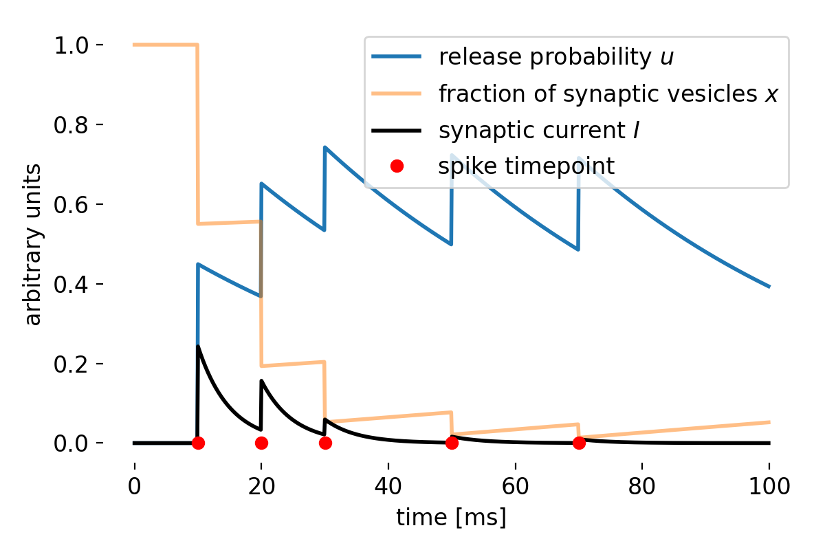 Simulated short-term depression (STD) in a synapse. A detailed explanation of the simulation is provided below.
Short-term depression (STD)
Short-term synaptic depression (STD) is a temporary decrease in synaptic strength that occurs when synapses are used repeatedly over a short period. This phenomenon reduces the likelihood of neurotransmitter release in response to subsequent stimuli.
The primary mechanism underlying STD is the depletion of the readily releasable pool of synaptic vesicles. When a synapse is activated rapidly, vesicles are released faster than they can be replenished, leading to a transient decrease in neurotransmitter release. Another contributing factor can be the temporary inactivation of the molecular machinery responsible for vesicle release.
In a simplified frequency-dependent interpretation, STD often acts more like a low-pass filter: Isolated or low-frequency presynaptic spikes are transmitted relatively effectively, whereas sustained high-frequency input progressively depletes the available synaptic resources and reduces the postsynaptic response. In this way, STD can support adaptation to sustained input, prevent excessive excitation, and emphasize changes in presynaptic activity rather than steady high-frequency drive.
Short-term facilitation (STF)
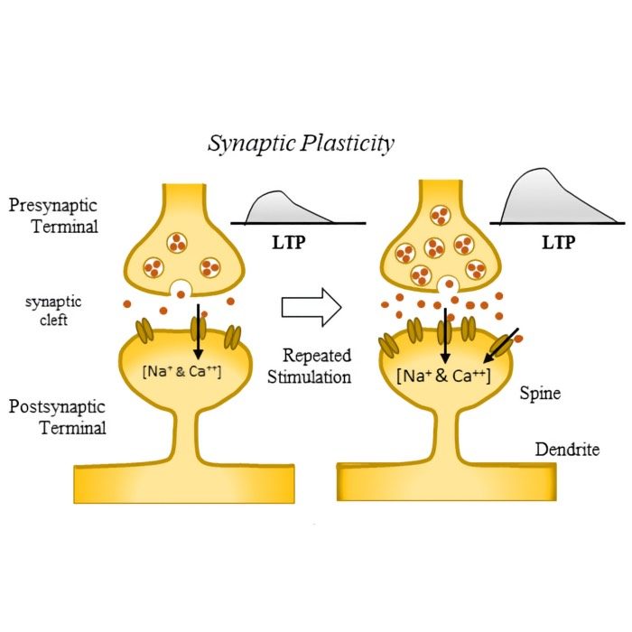
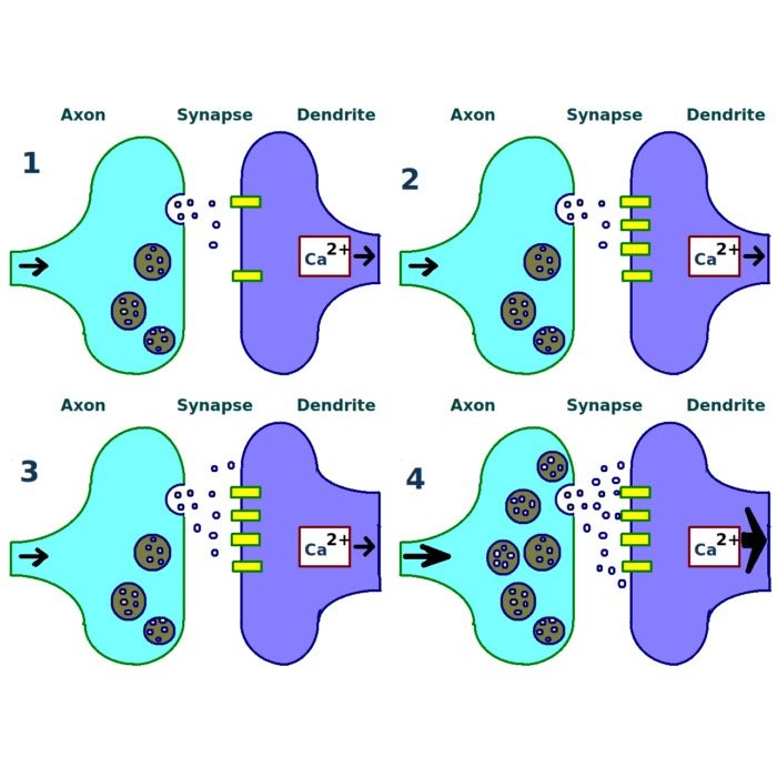
Short-term synaptic facilitation (STF) is a transient increase in synaptic strength that occurs when two or more action potentials invade the presynaptic terminal within a short time frame. This leads to an increased probability of neurotransmitter release in response to subsequent stimuli.
The most widely accepted mechanism for STF is the residual calcium hypothesis. When an action potential reaches the presynaptic terminal, it causes an influx of calcium ions (Ca2+). If another action potential arrives before the calcium is fully cleared, the residual calcium from the first spike adds to the influx from the second spike, increasing the probability of vesicle release. Short-term changes in the efficacy of the synaptic release machinery can also contribute to facilitation.
Again, in a simplified frequency-dependent interpretation, STF often acts more like a high-pass filter: Isolated presynaptic spikes evoke relatively small responses, whereas closely spaced spikes increase the release probability and thereby enhance subsequent postsynaptic responses. This makes facilitating synapses particularly sensitive to bursts or rapid sequences of action potentials and supports the temporal summation of synaptic inputs.
Interaction and implications
STD and STF often coexist at synapses, and their relative influence can vary based on the type of synapse and the pattern of neural activity. The balance between depression and facilitation can shape the overall dynamics of synaptic transmission and influence neural coding and network behavior. Their significance in neural processing can be summarized as follows:
- Both STD and STF contribute to the dynamic range modulation of synapses, allowing them to adjust their responsiveness based on recent activity.
- These forms of plasticity enable synapses to act as temporal filters, selectively enhancing or diminishing the transmission of specific patterns of activity.
- They play a role in maintaining synaptic homeostasis, ensuring that synaptic activity remains within a functional range and preventing overexcitation or underactivity.
Mathematical implementation
Both short-term depression and short-term facilitation can be mathematically modeled to capture their dynamics in neural networks. These models generally modify the synaptic efficacy based on the history of presynaptic activity. In 1998, Tsodyks and Markramꜛ proposed a phenomenological model that captures the essential features of both STD and STF. The model includes two variables, $x$ and $u$, which represent the synaptic depression and facilitation, respectively. The dynamics of these variables are governed by differential equations that depend on the presynaptic spike train and the synaptic parameters. Here are the detailed implementations of both mechanisms.
STD is modeled as a decrease in the fraction of available synaptic resources. The normalized fraction of available resources is denoted by $x$ ($0\leq x\leq1$): It is reduced at presynaptic spike times and recovers toward 1 between spikes with a time constant $\tau_d$. STF is modeled as an increase in the utilization of synaptic efficacy. The utilization factor is denoted by $u$: It increases at presynaptic spike times and, in the simplified convention used here, decays back toward 0 between spikes with a time constant $\tau_f$. The dynamics of $x$, $u$, and the synaptic current or conductance variable $I$ can be described by the following set of differential equations:
\[\begin{align} \frac{dx}{dt} &= \frac{1 - x}{\tau_d} - u^+ x^- \delta(t - t_{sp}) \\ \frac{du}{dt} &= -\frac{u}{\tau_f} + U(1 - u^-)\delta(t - t_{sp}) \label{eq:2} \\ \frac{dI}{dt} &= -\frac{I}{\tau_s} + A u^+ x^- \delta(t - t_{sp}) \end{align}\]where:
- $\tau_d$ is the depression time constant,
- $\tau_f$ is the facilitation time constant,
- $U$ is the utilization factor (a parameter that sets the fraction of resources used after each spike),
- $\delta(t - t_{sp})$ represents the Dirac delta function, indicating the occurrence of a presynaptic spike at time $t_{sp}$,
- $A$ is the amplitude of the synaptic response, and
- $I$ is the synaptic current or conductance.
Variables just before the arrival of a spike are denoted by the superscript $-$, and those just after the spike by the superscript $+$. From Eq. ($\ref{eq:2}$) we get:
\[\begin{align} u^+ &= u^- + U(1 - u^-) \\ x^+ &= x^- - u^+ x^- \end{align}\]After a spike, the variable $u$ increases by an amount proportional to $U$, reflecting the increased utilization of synaptic efficacy. Subsequently, a fraction $u^+$ of the currently available synaptic resources $x^-$ is used to generate the postsynaptic current or conductance increment. In the intervals between spikes, the simplified formulation used here lets $u$ decay back to zero with a time constant $\tau_f$, while $x$ gradually recovers to 1 with a time constant $\tau_d$. The synaptic current $I$ decays with a time constant $\tau_s$. When a spike occurs at $t_{sp}$, $x$ is reduced by an amount proportional to $u^+x^-$, and $I$ is incremented by a factor proportional to $Au^+x^-$.
It is worth noting that different formulations of the Tsodyks-Markram model use slightly different conventions for the facilitation variable. In the simplified pseudo-code implementation below, $u$ decays to zero between spikes. In other common formulations, including several simulator implementations, the utilization variable relaxes toward a baseline value related to $U$ instead. Therefore, the variables and parameters in this minimal implementation should not be compared one-to-one with those of every simulator implementation without checking the exact convention used there.
Pseudo-code implementation
It’s actually quite simple to implement the Tsodyks-Pawelzik-Markram model in Python. Let’s begin by importing the necessary libraries:
import numpy as np
import matplotlib.pyplot as plt

# Set global properties for all plots:
plt.rcParams.update({'font.size': 12})
plt.rcParams["axes.spines.top"]    = False
plt.rcParams["axes.spines.bottom"] = False
plt.rcParams["axes.spines.left"]   = False
plt.rcParams["axes.spines.right"]  = False
Next, we define the initial conditions and parameters for the simulation. To simulate a STD-dominating synapse, we can set the parameters as follows:
U_initial = 0.0 # set initial release probability
x_initial = 1.0 # set initial fraction of synaptic vesicles in the readily releasable pool

u = U_initial
x = x_initial
I = 0           # initial synaptic current in arbitrary units

# set time constants and parameters:
tau_f = 50   # facilitation time constant
tau_d = 750  # depression time constant
tau_s = 5    # synaptic current decay time constant
U = 0.45     # utilization factor
A = 1        # synaptic response amplitude
For a STF-dominating synapse, change the parameters as follows:
tau_f = 750  # facilitation time constant
tau_d = 50   # depression time constant
U     = 0.15 # utilization factor
We need to define the time step for numerical integration and the duration of the simulation. We also set some example spike times to observe the dynamics of the synapse:
# set time step for numerical integration:
dt = 0.1  # ms
simulation_duration = 100 # ms

# set some example spike times:
spike_times = [10, 20, 30, 50, 70]  # in ms
Finally, we simulate the dynamics of the synapse by iterating over time and updating the synaptic variables:
I_trace = []  # list to store the synaptic current over time
u_trace = []  # list to store the release probability over time
x_trace = []  # list to store the fraction of synaptic vesicles in the readily releasable pool over time

# simulation loop:
for t in np.arange(0, simulation_duration, dt):
    # check for spikes:
    if t in spike_times:
        # spike event:
        u = u + U * (1 - u)
        I = I + A * u * x
        x = x - u * x

    # update u, x, and I between spikes:
    u = u * np.exp(-dt/tau_f)    # exponential decay of facilitation
    x = x + (1 - x) * (dt/tau_d) # Euler step for recovery from depression
    I = I * np.exp(-dt/tau_s)    # exponential decay of synaptic current

    I_trace.append(I)
    u_trace.append(u)
    x_trace.append(x)
To visualize the results, we can plot the dynamics of the release probability $u$, the fraction of synaptic vesicles $x$, and the synaptic current $I$ over time:
time = np.arange(0, simulation_duration, dt)

# plot the results:
plt.figure(figsize=(6, 4))
plt.plot(time, u_trace, label="release probability $u$", lw=2.0)
plt.plot(time, x_trace, label="fraction of synaptic vesicles $x$", lw=2.0, alpha=0.5)
plt.plot(time, I_trace, label="synaptic current $I$", lw=2.0, c="black")
plt.plot(spike_times, np.zeros_like(spike_times), 'ro',label="spike timepoint")
plt.xlabel("time [ms]")
plt.ylabel(f"arbitrary units")
plt.legend()
plt.tight_layout()
plt.show()
In case of $\tau_d\gg\tau_f$ and a large $U$, the synapse exhibits STD-dominant behavior:
Simulation results for a STD-dominant synapse. Shown are the dynamics of the release probability $u$, the fraction of synaptic vesicles $x$, and the synaptic current $I$ over time. We set $\tau_d=750$, $\tau_f=50$, $U=0.45$, $A=1$, $U_{\text{initial}}=0$, and $x_{\text{initial}}=1$ for this simulation.
In this STD-dominated parameter regime, the available-resource variable $x$ is progressively depleted by repeated spikes and recovers only slowly. Although $u$ may transiently increase at spike times, the product $ux$, and hence the effective synaptic response, decreases across the spike train. The synapse therefore becomes less responsive to subsequent spikes, reflecting the effects of short-term depression.
In case of $\tau_f\gg\tau_d$ and a small $U$, the synapse exhibits STF-dominant behavior:
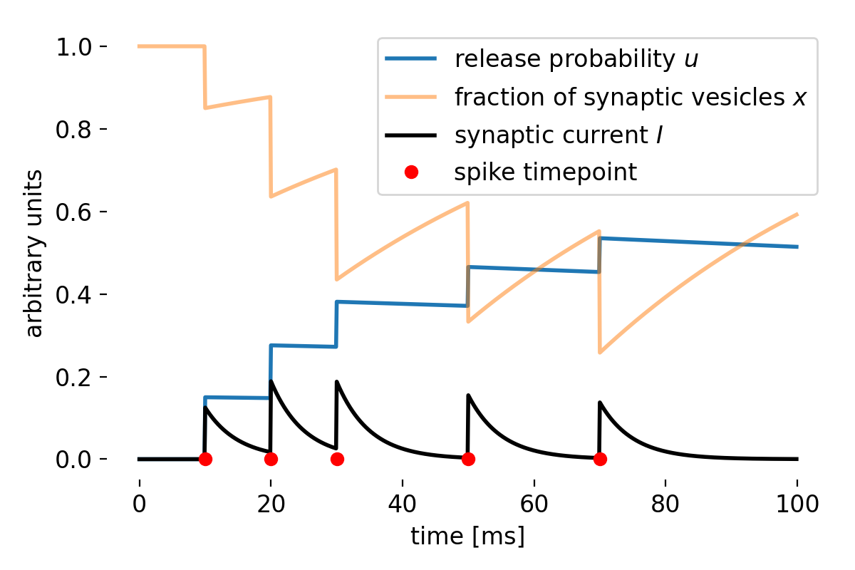
Same plot as before, but now for a STF-dominant synapse. We set $\tau_d=50$, $\tau_f=750$, $U=0.15$, $A=1$, $U_{\text{initial}}=0$, and $x_{\text{initial}}=1$.
In this STF-dominated parameter regime, the facilitation variable $u$ increases across closely spaced spikes, while the available-resource variable $x$ recovers relatively quickly. As a result, the product $ux$, and hence the effective synaptic response, increases across the spike train. The synapse therefore becomes more responsive to subsequent spikes, reflecting the effects of short-term facilitation.
Thus, the actual interplay between the dynamics of $x$ and $u$ determines whether the combined effect of $ux$ is dominated by depression or facilitation.
Simulation in NEST
NEST’s iaf_tum_2000ꜛ model includes a built-in implementation of short-term plasticity according to the Tsodyks-Uziel-Markram model proposed in 2000ꜛ. In the example below, the short-term plasticity variables are part of the iaf_tum_2000 neuron model, while the connection between the two neurons is created using a static_synapse. Thus, the term “synapse” in the following refers to the effective dynamic synaptic response generated by the model, not to a separate dynamic synapse object. For simulations in which short-term plasticity should be attached explicitly to synaptic connections, NEST also provides dedicated synapse models such as tsodyks_synapseꜛ.
Here is an example of how to simulate both STD and STF in NEST, following the NEST tutorials “Short-term facilitation example”ꜛ and “Short-term depression example”ꜛ with some minor modifications.
import matplotlib.pyplot as plt
import numpy as np
import nest

# set the verbosity of the NEST simulator:
nest.set_verbosity("M_WARNING")

# Set global properties for all plots:
plt.rcParams.update({'font.size': 12})
plt.rcParams["axes.spines.top"]    = False
plt.rcParams["axes.spines.bottom"] = False
plt.rcParams["axes.spines.left"]   = False
plt.rcParams["axes.spines.right"]  = False
We begin by simulating an effective synaptic response with short-term depression (STD). We set the parameters of the iaf_tum_2000 model and the simulation duration. We also define the DC input amplitude and frequency, as well as the initial values for the short-term plasticity variables $x$ and $u$:
nest.ResetKernel()
nest.resolution = 0.1  # simulation step size [ms]

T_sim = 1200.0  # simulation time [ms]

tau_m = 40.0  # membrane time constant [ms]
R_m = 0.1  # membrane input resistance [GΩ]
C_m = tau_m / R_m  # membrane capacitance [pF]
V_th = 15.0  # threshold potential [mV]
V_reset = 0.0  # reset potential [mV]
t_ref = 2.0  # refractory period [ms]

stim_start = 50.0   # start time of DC input [ms]
stim_end   = 1050.0 # end time of DC input [ms]
f_hz       = 20.0   # frequency [Hz]
f = f_hz / 1000.0   # frequency conversion to [1/ms]
dc_amp = V_th * C_m / tau_m / (1 - np.exp(-(1 / f - t_ref) / tau_m))  # DC amplitude [pA]

dc_gen = nest.Create("dc_generator", 1,
                     params={"amplitude": dc_amp,
                             "start": stim_start,
                             "stop": stim_end})

x = 1.0  # initial fraction of synaptic vesicles in the readily releasable pool
u = 0.0  # initial release probability of synaptic vesicles
U = 0.5  # fraction determining the increase in u with each spike
tau_psc = 3.0  # decay constant of PSCs (tau_inact in [2]) [ms]
tau_rec = 800.0  # recovery time from synaptic depression [ms]
tau_fac = 0.0  # time constant for facilitation (off) [ms]
Next, we create two neurons with the iaf_tum_2000 model and connect them using a static_synapse. Note that the short-term depression dynamics are not implemented by the static_synapse itself, but by the short-term plasticity variables inside the iaf_tum_2000 model. We also create a multimeter to record the membrane potential and synaptic currents:
neurons = nest.Create("iaf_tum_2000", 2, params={
                    "C_m": C_m,
                    "tau_m": tau_m,
                    "tau_syn_ex": tau_psc,
                    "tau_syn_in": tau_psc,
                    "V_th": V_th,
                    "V_reset": V_reset,
                    "E_L": V_reset,
                    "V_m": V_reset,
                    "t_ref": t_ref,
                    "U": U,
                    "tau_psc": tau_psc,
                    "tau_rec": tau_rec,
                    "tau_fac": tau_fac,
                    "x": x,
                    "u": u})

nest.Connect(dc_gen, neurons[0])

weight = 250.0  # synaptic weight [pA]
delay = 0.1  # synaptic delay [ms]

nest.Connect(neurons[0], neurons[1], syn_spec={
                "synapse_model": "static_synapse",
                "weight": weight,
                "delay": delay,
                "receptor_type": 1})

multimeter_std = nest.Create("multimeter",
                             params={"interval": 1.0,
                                     "record_from": ["V_m", 'I_syn_ex', 'I_syn_in']})
nest.Connect(multimeter_std, neurons[1])
Finally, we simulate the network and extract the recordings from the multimeter (we will plot them later):
nest.Simulate(T_sim)

# extract recordings from the multimeter:
times_STD = multimeter_std.get("events")["times"]
I_syn_ex_STD = multimeter_std.get("events")["I_syn_ex"]
I_syn_in_STD = multimeter_std.get("events")["I_syn_in"]
V_m_STD = multimeter_std.get("events")["V_m"]
Next, we simulate an effective synaptic response with short-term facilitation (STF) using the same procedure. We set the parameters of the iaf_tum_2000 model and the simulation duration, as well as the initial values for the short-term plasticity variables $x$ and $u$:
nest.ResetKernel()
nest.resolution = 0.1  # simulation step size [ms]

dc_gen = nest.Create("dc_generator", 1,
                     params={"amplitude": dc_amp,
                             "start": stim_start,
                             "stop": stim_end})

x = 1.0  # initial fraction of synaptic vesicles in the readily releasable pool
u = 0.0  # initial release probability of synaptic vesicles
U = 0.03  # fraction determining the increase in u with each spike
tau_psc = 1.5  # decay constant of PSCs (tau_inact in [2]) [ms]
tau_rec = 130.0  # recovery time from synaptic depression [ms]
tau_fac = 530.0  # time constant for facilitation [ms]

neurons = nest.Create("iaf_tum_2000", 2,params={
                    "C_m": C_m,
                    "tau_m": tau_m,
                    "tau_syn_ex": tau_psc,
                    "tau_syn_in": tau_psc,
                    "V_th": V_th,
                    "V_reset": V_reset,
                    "E_L": V_reset,
                    "V_m": V_reset,
                    "t_ref": t_ref,
                    "U": U,
                    "tau_psc": tau_psc,
                    "tau_rec": tau_rec,
                    "tau_fac": tau_fac,
                    "x": x,
                    "u": u})

nest.Connect(dc_gen, neurons[0])

weight = 1540.0  # synaptic weight [pA]
delay = 0.1  # synaptic delay [ms]

nest.Connect(neurons[0], neurons[1], syn_spec={
                "synapse_model": "static_synapse",
                "weight": weight,
                "delay": delay,
                "receptor_type": 1})

multimeter_stf = nest.Create("multimeter",
                             params={"interval": 1.0,
                                     "record_from": ["V_m", 'I_syn_ex', 'I_syn_in']})
nest.Connect(multimeter_stf, neurons[1])

nest.Simulate(T_sim)

# extract voltage trace from the voltmeter and plot it:
times_STF = multimeter_stf.get("events")["times"]
I_syn_ex_STF = multimeter_stf.get("events")["I_syn_ex"]
I_syn_in_STF = multimeter_stf.get("events")["I_syn_in"]
V_m_STF = multimeter_stf.get("events")["V_m"]
Finally, we plot the results for both STD and STF simulations:
fig1, ax = plt.subplots(2, 1, sharex=True, figsize=(6.5, 5))

ax[0].plot(times_STD, V_m_STD, label="V_m (STD)")
ax[0].plot(times_STF, V_m_STF, label="V_m (STF)", alpha=0.5)
ax[0].legend()
ax[0].set_ylabel(f"membrane potential\n[mV]")

ax[1].plot(times_STD, I_syn_ex_STD, label="I_syn_ex (STD)")
ax[1].plot(times_STF, I_syn_ex_STF, label="I_syn_ex (STF)", alpha=0.5)
ax[1].legend()
ax[1].set_xlabel("time [ms]")
ax[1].set_ylabel(f"synaptic current\n[pA]")

plt.tight_layout()
plt.show()
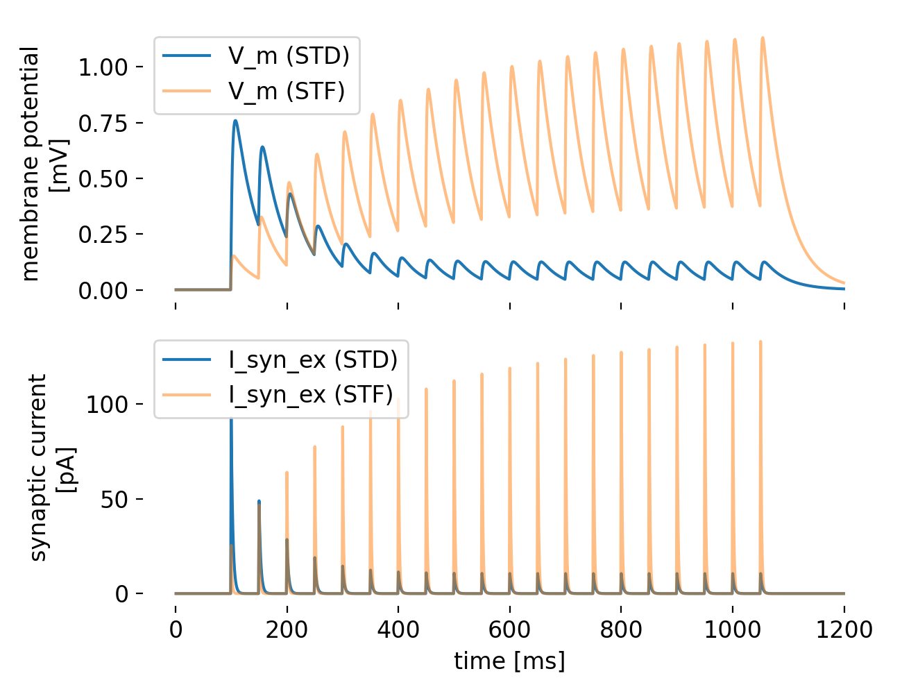
Simulation results for a synapse with short-term depression (STD, blue) and short-term facilitation (STF, orange). The top panel shows the membrane potential $V_m$ of the postsynaptic neuron, while the bottom panel shows the excitatory synaptic current $I_{\text{syn_ex}}$. The STD synapse exhibits a transient decrease in synaptic current after each spike, while the STF synapse shows an increase in synaptic current after each spike. The DC input is applied from 50 ms to 1050 ms.
The plot shows the membrane potential $V_m$ of the postsynaptic neuron and the excitatory synaptic current $I_{\text{syn_ex}}$ for both the STD (blue) and STF (orange) synapses. The STD synapse exhibits a rapid initial increase in $V_m$ due to the synaptic input, followed by a gradual decrease as the depression mechanism reduces the synaptic efficacy. In case of the STF synapse, $V_m$ continues to increase with successive spikes due to the facilitation mechanism, which increases synaptic efficacy. Both observations are consistent with the expected behavior of STD and STF, respectively. This is also reflected in the synaptic current $I_{\text{syn_ex}}$, which shows a transient decrease after each spike for the STD synapse (STD causes the depletion of available synaptic resources with each spike) and a transient increase for the STF synapse (with each successive spike, STF enhances the release probability in this case).
Overall, this simulation illustrated the contrasting effects of short-term depression and facilitation on synaptic plasticity, demonstrating how these mechanisms can dynamically modulate neural responses based on spike timing and frequency.
Conclusion
Short-term depression (STD) and short-term facilitation (STF) are essential mechanisms of short-term synaptic plasticity that regulate the strength of synaptic transmission in response to presynaptic activity. These mechanisms play crucial roles in shaping neural responses, filtering information, and maintaining synaptic homeostasis. By implementing STD and STF in computational models of neural networks, we can study their effects on network dynamics, information processing, and learning. The Tsodyks-Pawelzik-Markram model provides a simple yet effective framework for capturing the dynamics of STD and STF, allowing us to simulate and analyze the behavior of synapses under different conditions. By combining experimental and computational approaches, we can gain a deeper understanding of how short-term plasticity influences neural function and network behavior.
The complete code used in this blog post is available in this Github repositoryꜛ (short_term_synaptic_plasticity.py and short_term_synaptic_plasticity_with_NEST.py). Feel free to modify and expand upon it, and share your insights.
References
- Zucker, Regehr, Short-Term Synaptic Plasticity, 2002, Annual Review of Physiology, Vol. 64, Issue 1, pages 355-405, doi: 10.1146/annurev.physiol.64.092501.114547ꜛ
- L. F. Abbott, Wade G. Regehr, Synaptic computation, 2004, Nature, Vol. 431, Issue 7010, pages 796-803, doi: doi.org/10.1038/nature03010
- L. F. Abbott, S. B. Nelson, Synaptic plasticity: taming the beast, 2000, Nature neuroscience, doi: 10.1038/81453ꜛ
- Misha Tsodyks, Klaus Pawelzik, Henry Markram, Neural Networks with Dynamic Synapses, 1998, Neural Computation, Vol. 10, Issue 4, pages 821-835, doi: 10.1162/089976698300017502ꜛ
- Misha Tsodyks, Asher Uziel, Henry Markram, Synchrony Generation in Recurrent Networks with Frequency-Dependent Synapses, 2000, The Journal of Neuroscience, Vol. 20, Issue 1, pages RC50-RC50, doi: 10.1523/JNEUROSCI.20-01-j0003.2000ꜛ
- Citri, Malenka, Synaptic Plasticity: Multiple Forms, Functions, and Mechanisms, 2008, Neuropsychopharmacology, Vol. 33, Issue 1, pages 18-41, doi: 10.1038/sj.npp.1301559
- scholarpedia article on ‘Short-term synaptic plasticity’ꜛ
- NEST’s
iaf_tum_2000model descriptionꜛ - NEST’s
tsodyks_synapsemodel descriptionꜛ - NEST’s “Short-term facilitation example” tutorialꜛ
- NEST’s “Short-term depression example” tutorialꜛ
comments