Clopath plasticity rule

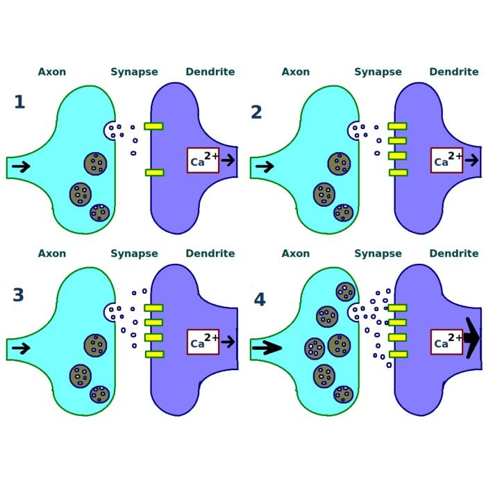
The Clopath learning rule is a biophysically inspired model of synaptic plasticity that extends classical Hebbian learning and simple spike-timing-dependent plasticity (STDP) formulations by incorporating the postsynaptic membrane voltage as an explicit state variable. Introduced by Claudia Clopath et al. in 2010ꜛ, the rule was designed to account for experimental findings that cannot be captured well by timing-only STDP rules. In particular, synaptic potentiation and depression do not depend only on the relative timing of pre- and postsynaptic spikes, but also on the depolarization state of the postsynaptic neuron.

Result of a spike pairing simulation using the Clopath rule. The plot shows the change in synaptic weight as a function of the relative timing of pre- and postsynaptic spikes. The Clopath rule captures both potentiation and depression of synaptic weights based on the timing of spikes and the postsynaptic membrane potential. We will simulate this experiment in the section “Spike pairing simulation” below.

This makes the Clopath rule especially important in computational neuroscience. It provides a compact phenomenological framework that links synaptic plasticity to membrane dynamics, spike timing, and homeostatic stabilization. As a result, it is widely used in spiking neural network simulations that aim to remain closer to biological plasticity mechanisms than pair-based STDP rules.

Mathematical description

The central idea of the Clopath rule is that potentiation and depression depend on different combinations of presynaptic activity and postsynaptic voltage. In contrast to simple STDP rules, the postsynaptic membrane potential is not treated as an implicit byproduct of spike times, but as a relevant dynamical quantity in its own right.

A simplified schematic form of the rule can be written as

\[\begin{align*} \frac{dw_{ij}}{dt} =& -A_\text{LTD} \, x_i(t)\,[\bar{u}_j(t)-\theta_-]_+ \\ & + A_\text{LTP} \, \bar{x}_i(t)\,[u_j(t)-\theta_+]_+[\bar{u}_j(t)-\theta_-]_+, \end{align*}\]

where

• $w_{ij}$ is the synaptic weight from presynaptic neuron $i$ to postsynaptic neuron $j$,
• $A_\text{LTD}$ and $A_\text{LTP}$ set the relative strength of the depressive and potentiating plasticity components,
• $x_i(t)$ and $\bar{x}_i(t)$ are presynaptic traces,
• $u_j(t)$ is the postsynaptic membrane potential,
• $\bar{u}_j(t)$ is a low pass filtered postsynaptic voltage,
• $\theta_-$ and $\theta_+$ are voltage thresholds for depression and potentiation, respectively, and
• $[\,\cdot\,]_+ = \max(\cdot,0)$ denotes rectification.

This expression captures the main logic of the model:

• depression is triggered when presynaptic activity coincides with sufficient postsynaptic depolarization above a lower threshold
• potentiation requires stronger postsynaptic depolarization above a higher threshold and depends on presynaptic activation through a trace term
• the two processes are therefore asymmetric in their voltage dependence

The precise formulation differs somewhat between the original papers and specific simulator implementations such as NEST (see below), but the conceptual structure remains the same.

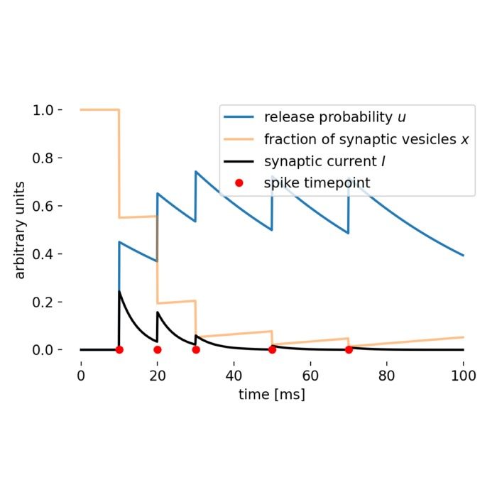
A typical presynaptic trace is described by

\[\frac{dx_i(t)}{dt} = -\frac{x_i(t)}{\tau_x} + \sum_f \delta(t-t_i^f),\]

where $\tau_x$ is the decay time constant and $t_i^f$ denotes the times of presynaptic spikes. $\delta(t - t_i^f)$ represents the Dirac delta function indicating a presynaptic spike at time $t_i^f$. $f$ denotes the time of the presynaptic spike. The (low-pass) filtered postsynaptic voltage potential can be written as

\[\frac{d\bar{u}_j(t)}{dt} = -\frac{\bar{u}_j(t)}{\tau_u} + u_j(t),\]

where $\tau_u$ is the corresponding voltage filter (decay) time constant.

In addition to its voltage dependence, the original Clopath model also contains a homeostatic component that prevents runaway synaptic growth. This is one of the key reasons why the rule is more stable in recurrent network simulations than many simpler STDP variants.

The synaptic weights are typically bounded such that

\[0 \leq w_{ij} \leq w_\text{max}.\]

In some versions of the model, the LTD amplitude is further modulated by a homeostatic postsynaptic activity term, for example in the schematic form

\[A_\text{LTD} \propto \alpha \frac{\bar{u}_{j,\mathrm{homeo}}^2}{u_\text{ref}^2},\]

where $\alpha$ is a scaling factor, $u_\text{ref}$ is a reference level, and $\bar{u}_{j,\mathrm{homeo}}$ denotes a slowly varying postsynaptic activity or voltage measure rather than the instantaneous membrane potential itself. The exact form depends on the specific model variant or simulator implementation. This allows the rule to counteract runaway potentiation and helps maintain stable learning in recurrent networks.

Implementation in neural network simulations

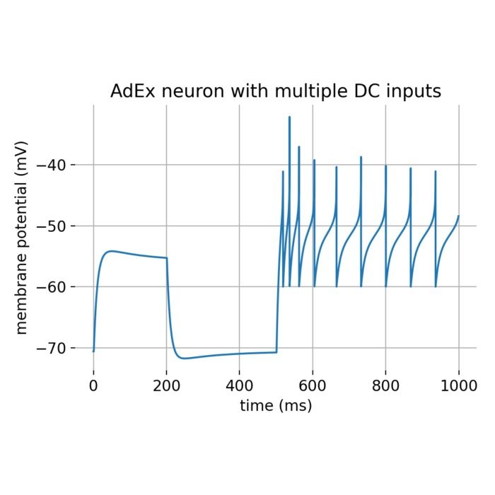
To use the Clopath rule in a spiking network simulation, one must supply not only pre- and postsynaptic spikes but also the postsynaptic membrane voltage and its filtered versions. For this reason, the rule is often coupled to a neuron model that provides a realistic subthreshold voltage trajectory. A common choice is the adaptive exponential integrate and fire (AdEx) neuron model, which captures leak dynamics, exponential spike initiation, and adaptation. A standard AdEx membrane equation is

\[\begin{align*} C \frac{du(t)}{dt} = & -g_L \bigl(u(t)-E_L\bigr) + g_L \Delta_T e^{(u(t)-V_T)/\Delta_T} \\ & - I_\text{adapt}(t) + I_\text{syn}(t) + I_\text{ext}(t), \end{align*}\]

where $u(t)$ is the membrane potential, $C$ is the membrane capacitance, $g_L$ is the leak conductance, $E_L$ is the resting potential, $\Delta_T$ controls the sharpness of spike initiation, $V_T$ is the (adaptive) threshold parameter, $I_\text{adapt}(t)$ is the adaptation current, $I_\text{syn}(t)$ is the synaptic current, and $I_\text{ext}(t)$ is the external input current.

The adaptation current is commonly modeled as

\[\frac{dI_\text{adapt}(t)}{dt} = \frac{a\bigl(u(t)-E_L\bigr)-I_\text{adapt}(t)}{\tau_\text{adapt}},\]

where $a$ is the adaptation conductance and $\tau_\text{adapt}$ is the adaptation time constant.

In the context of the Clopath rule, the synaptic current $I_\text{syn}(t)$ is given by the sum of inputs from all presynaptic neurons, weighted by their synaptic weights $w_{ij}$:

\[I_\text{syn}(t) = \sum_i w_{ij} \cdot x_i(t).\]

In this setting, the Clopath synapse does not replace the neuron model. Rather, it uses the neuron model’s voltage trajectory to determine when synaptic potentiation or depression should occur. This separation is important conceptually: The AdEx model describes membrane dynamics, whereas the Clopath rule describes plasticity at synapses.

In some AdEx-based implementations, the threshold potential is itself adaptive and evolves dynamically after each spike. A simple phenomenological form is

\[\frac{dV_T(t)}{dt} = -\frac{V_T(t)-V_{T,\infty}}{\tau_{V_T}},\]

where $V_{T,\infty}$ is the baseline threshold value and $\tau_{V_T}$ is the corresponding relaxation time constant.

In Clopath and Gerstner (2010)ꜛ, the interaction between spike timing and voltage was further analyzed in a formulation that includes a depolarizing spike afterpotential. This can be represented by an additional variable $z(t)$ that is incremented at spike times and otherwise decays exponentially:

\[\frac{dz(t)}{dt} = -\frac{z(t)}{\tau_z}.\]

Such additions are useful because they help reproduce experimental pairing protocols more faithfully.

Why the Clopath rule matters

The Clopath learning rule is significant for several reasons:

Biological plausibility

A major advantage of the Clopath rule is that it links synaptic modification to the postsynaptic voltage state. This reflects the fact that in biological neurons, synaptic plasticity is shaped not only by spike timing but also by dendritic and somatic depolarization. In this sense, the rule is substantially closer to experimentally observed plasticity than purely timing-based STDP models.

Voltage dependence

The model distinguishes between weaker depolarization regimes associated with depression and stronger depolarization regimes associated with potentiation. This captures an important principle of real synapses: The effect of presynaptic input depends on the electrical state of the postsynaptic cell. The same presynaptic spike train can therefore induce very different weight changes depending on whether the postsynaptic neuron is weakly depolarized, strongly depolarized, or near firing threshold.

Homeostasis

The Clopath model includes homeostatic ingredients that help constrain weight growth and maintain stable activity over time. This is especially important in recurrent networks (RNN), where unconstrained Hebbian plasticity can otherwise produce runaway excitation or pathological synchrony.

Computational usefulness

From a modeling perspective, the Clopath rule is attractive because it remains relatively compact while capturing several important experimental dependencies. In particular, it provides a practical compromise between biological realism and computational tractability: It goes beyond purely timing-based STDP rules by incorporating postsynaptic voltage, yet remains simple enough to be used in larger spiking network simulations. This makes it useful in studies of receptive field formation, self-organization, synaptic competition, and activity-dependent structure in recurrent circuits. Because each synapse is updated locally on the basis of presynaptic activity and the postsynaptic voltage state, even reciprocal connections between two neurons do not have to evolve symmetrically. In this way, the rule can contribute to the emergence of structured and direction-specific connectivity patterns rather than merely uniform global weight changes. Whenever a plasticity model is needed that depends on more than spike timing alone, the Clopath rule is a natural candidate.

Spike pairing simulation

The Clopath rule (clopath_synapseꜛ) and the corresponding voltage-based neuron model (aeif_psc_delta_clopathꜛ) are both implemented in the NEST simulator. To illustrate the behavior of the rule, we can reproduce the NEST tutorial “Clopath Rule: Spike pairing experiment”ꜛ. The goal is to study how synaptic weights change under repeated spike pairings with different temporal structure and different effective pairing frequencies.

Let’s start by importing the necessary libraries:

import matplotlib.pyplot as plt
import numpy as np
import nest

# set the verbosity of the NEST simulator:
nest.set_verbosity("M_WARNING")

# Set global properties for all plots
plt.rcParams.update({'font.size': 12})
plt.rcParams["axes.spines.top"]    = False
plt.rcParams["axes.spines.bottom"] = False
plt.rcParams["axes.spines.left"]   = False
plt.rcParams["axes.spines.right"]  = False

nest.ResetKernel()

# define the simulation resolution:
resolution = 0.1

Next, we define the parameters of the neuron.,

# define the parameters of the neuron:
clopath_neuron_params = {
    "V_m": -70.6,           # [mV] membrane potential
    "E_L": -70.6,           # [mV] leak reversal potential
    "C_m": 281.0,           # [pF] membrane capacitance
    "theta_minus": -70.6,   # [mV] threshold for u (LTD)
    "theta_plus": -45.3,    # [mV] threshold for u_bar (LTP)
    "A_LTD": 14.0e-5,       # [nS] amplitude of LTD
    "A_LTP": 8.0e-5,        # [nS] amplitude of LTP
    "tau_u_bar_minus": 10.0,# [ms] time constant for u_bar_minus (LTD)
    "tau_u_bar_plus": 7.0,  # [ms] time constant for u_bar_plus (LTP)
    "delay_u_bars": 4.0,    # [ms] delay with which u_bar_[plus/minus] are processed to compute the synaptic weights.
    "a": 4.0,               # [nS] subthreshold adaptation
    "b": 0.0805,            # [pA] spike-triggered adaptation
    "V_reset": -70.6 + 21.0,# [mV] reset potential
    "V_clamp": 33.0,        # [mV] clamping potential
    "t_clamp": 2.0,         # [ms] clamping time
    "t_ref": 0.0,           # [ms] refractory period
}

We then need to define the spike times for the pre- and postsynaptic neurons. They are arranged in two lists, spike_times_pre and spike_times_post, each containing the spike times for different pairs of pre- and postsynaptic neurons. The simulation will run for each pair of spike times:

spike_times_pre = [
    # Presynaptic spike before the postsynaptic
    [20.0, 120.0, 220.0, 320.0, 420.0],
    [20.0, 70.0, 120.0, 170.0, 220.0],
    [20.0, 53.3, 86.7, 120.0, 153.3],
    [20.0, 45.0, 70.0, 95.0, 120.0],
    [20.0, 40.0, 60.0, 80.0, 100.0],
    # Presynaptic spike after the postsynaptic
    [120.0, 220.0, 320.0, 420.0, 520.0, 620.0],
    [70.0, 120.0, 170.0, 220.0, 270.0, 320.0],
    [53.3, 86.6, 120.0, 153.3, 186.6, 220.0],
    [45.0, 70.0, 95.0, 120.0, 145.0, 170.0],
    [40.0, 60.0, 80.0, 100.0, 120.0, 140.0]]

spike_times_post = [
    [10.0, 110.0, 210.0, 310.0, 410.0],
    [10.0, 60.0, 110.0, 160.0, 210.0],
    [10.0, 43.3, 76.7, 110.0, 143.3],
    [10.0, 35.0, 60.0, 85.0, 110.0],
    [10.0, 30.0, 50.0, 70.0, 90.0],
    [130.0, 230.0, 330.0, 430.0, 530.0, 630.0],
    [80.0, 130.0, 180.0, 230.0, 280.0, 330.0],
    [63.3, 96.6, 130.0, 163.3, 196.6, 230.0],
    [55.0, 80.0, 105.0, 130.0, 155.0, 180.0],
    [50.0, 70.0, 90.0, 110.0, 130.0, 150.0]]

We set the initial weight of the synapse,

# set the initial weight of the synapse::
init_w = 0.5
syn_weights = []

and run the simulation for each pair of spike times (the weights are recorded for each simulation run):

for s_t_pre, s_t_post in zip(spike_times_pre, spike_times_post):
    nest.ResetKernel()
    nest.resolution = resolution

    # create one adaptive exponential integrate-and-fire neuron neuron with Clopath synapse:
    clopath_neuron = nest.Create("aeif_psc_delta_clopath", 1, clopath_neuron_params)

    # We need a parrot neuron for technical reasons since spike generators can only
    # be connected with static connections:
    parrot_neuron = nest.Create("parrot_neuron", 1)

    # create and connect spike generators:
    spike_gen_pre = nest.Create("spike_generator", {"spike_times": s_t_pre})
    nest.Connect(spike_gen_pre, parrot_neuron, syn_spec={"delay": resolution})

    spike_gen_post = nest.Create("spike_generator", {"spike_times": s_t_post})
    nest.Connect(spike_gen_post, clopath_neuron, syn_spec={"delay": resolution, "weight": 80.0})

    # create weight recorder:
    weightrecorder = nest.Create("weight_recorder")

    # create Clopath connection with weight recorder:
    nest.CopyModel("clopath_synapse", "clopath_synapse_rec", {"weight_recorder": weightrecorder})
    syn_dict = {"synapse_model": "clopath_synapse_rec", "weight": init_w, "delay": resolution}
    nest.Connect(parrot_neuron, clopath_neuron, syn_spec=syn_dict)

    # simulation:
    simulation_time = 10.0 + max(s_t_pre[-1], s_t_post[-1])
    nest.Simulate(simulation_time)

    # extract and save synaptic weights:
    weights = weightrecorder.get("events", "weights")
    syn_weights.append(weights[-1])

syn_weights = np.array(syn_weights)
# scaling of the weights so that they are comparable to Clopath et al (2010):
syn_weights = 100.0 * 15.0 * (syn_weights - init_w) / init_w + 100.0

Finally, we plot the results:

plt.figure(figsize=(4.5, 3.5))
plt.plot([10.0, 20.0, 30.0, 40.0, 50.0], syn_weights[5:], 
         lw=2.5, ls="-", label="pre-post pairing")
plt.plot([10.0, 20.0, 30.0, 40.0, 50.0], syn_weights[:5], 
         lw=2.5, ls="-", label="post-pre pairing")
plt.ylabel("normalized weight change")
plt.xlabel("firing rate of the presynaptic neuron [Hz]")
plt.legend()
plt.title(f"Synaptic weight using\nthe Clopath rule")
plt.tight_layout()
plt.show()

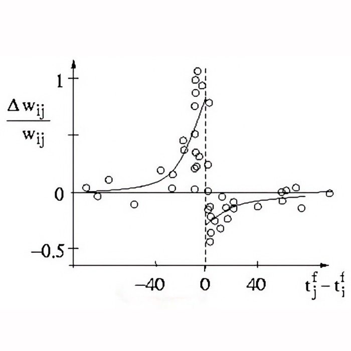
The resulting plot shows the synaptic weight change for different pairs of pre- and postsynaptic spike timings, plotted as a function of the firing rate of the presynaptic neuron. It shows how weight change depends not only on the order of spikes but also on the repetition frequency of the pairing protocol:

Synaptic weight change using the Clopath rule for different pairs of pre- and postsynaptic spike timings. The weight change is normalized to the initial weight and scaled to be comparable to Clopath et al. (2010)ꜛ. The two curves correspond to different temporal pairing orders and illustrate that the outcome depends jointly on spike timing, voltage dynamics, and repetition frequency.

The key observations in this plot are:

• pre-post pairing: As the firing rate of the presynaptic neuron increases, the synaptic weight change also increases. This indicates stronger synaptic potentiation at higher firing rates.
• post-pre pairing: The synaptic weight change increases similarly with higher firing rates but at lower rates compared to pre-post pairing. This shows a tendency for less potentiation or even depression in this pairing scenario for lower frequencies. However, for higher frequencies, the difference between pre-post and post-pre pairings diminishes.

The frequency of presynaptic spikes is crucial because it can significantly impact the degree of synaptic plasticity. Higher frequencies typically lead to more substantial changes in synaptic weights due to increased temporal overlap between pre- and postsynaptic spikes, which enhances the effects of spike-timing-dependent plasticity (STDP).

Network simulation of bidirectional connections

Next, we further investigate the Clopath rule by recapitulating the NEST tutorial “Clopath Rule: Large network simulation with bidirectional connections”ꜛ. In this simulation, we create a recurrent network of 10 excitatory and 3 inhibitory neurons connected with Clopath synapses, stimulated by Poisson generators. The goal is not to examine isolated spike pairs, but to see how voltage-based synaptic plasticity shapes connectivity within a small network of excitatory neurons embedded in an input driven circuit.

Let’s begin by importing the necessary libraries and setting the simulation parameters:

import random
import matplotlib.pyplot as plt
from mpl_toolkits.axes_grid1 import make_axes_locatable
import numpy as np
import nest

# set the verbosity of the NEST simulator:
nest.set_verbosity("M_WARNING")

# Set global properties for all plots
plt.rcParams.update({'font.size': 12})
plt.rcParams["axes.spines.top"]    = False
plt.rcParams["axes.spines.bottom"] = False
plt.rcParams["axes.spines.left"]   = False
plt.rcParams["axes.spines.right"]  = False


# set the simulation resolution and time:
simulation_time = 1.0e4
resolution = 0.1
delay = resolution
nest.ResetKernel()
nest.resolution = resolution

# for reproducibility:
np.random.seed(1)

Next, we define the parameters of the Clopath synapse and the neuron model and make connections between the neurons in the network. We create 10 excitatory and 3 inhibitory neurons and connect them with Clopath synapses. We also create Poisson generators to stimulate the network by 500 input neurons:

# poisson_generator parameters:
pg_A = 30.0     # amplitude of Gaussian
pg_sigma = 10.0 # std deviation

# create neurons and devices:
nrn_model = "aeif_psc_delta_clopath"
nrn_params = {
    "V_m": -30.6,           # [mV] membrane potential
    "g_L": 30.0,            # [nS] leak conductance
    "w": 0.0,               # [nS] adaptation conductance
    "tau_u_bar_plus": 7.0,  # [ms] time constant for u_bar_plus (LTP)
    "tau_u_bar_minus": 10.0,# [ms] time constant for u_bar_minus (LTD)
    "tau_w": 144.0,         # [ms] time constant for w
    "a": 4.0,               # [nS] subthreshold adaptation conductance
    "C_m": 281.0,           # [pF] membrane capacitance
    "Delta_T": 2.0,         # [mV] slope factor
    "V_peak": 20.0,         # [mV] spike cut-off
    "t_clamp": 2.0,         # [ms] clamping time
    "A_LTP": 8.0e-6,        # [nS] amplitude of LTP
    "A_LTD": 14.0e-6,       # [nS] amplitude of LTD
    "A_LTD_const": False,   
    "b": 0.0805,            # [nA] spike-triggered adaptation
    "u_ref_squared": 60.0**2# [nA^2] squared threshold for u
    }

pop_exc = nest.Create(nrn_model, 10, nrn_params) # create 10 excitatory neurons
pop_inh = nest.Create(nrn_model, 3, nrn_params)  # create 3 inhibitory neurons

pop_input = nest.Create("parrot_neuron", 500)    # helper neurons (for technical reasons)
pg = nest.Create("poisson_generator", 500)       # poisson generators; i.e., 500 input neurons
wr = nest.Create("weight_recorder")              # create a weight recorder

nest.Connect(pg, pop_input, "one_to_one", 
             {"synapse_model": "static_synapse", 
              "weight": 1.0, 
              "delay": delay})

nest.CopyModel("clopath_synapse", "clopath_input_to_exc", {"Wmax": 3.0})
conn_dict_input_to_exc = {"rule": "all_to_all"}
syn_dict_input_to_exc = {"synapse_model": "clopath_input_to_exc",
                         "weight": nest.random.uniform(0.5, 2.0),
                         "delay": delay}
nest.Connect(pop_input, pop_exc, conn_dict_input_to_exc, syn_dict_input_to_exc)

# create input->inh connections:
conn_dict_input_to_inh = {"rule": "all_to_all"}
syn_dict_input_to_inh = {"synapse_model": "static_synapse", "weight": nest.random.uniform(0.0, 0.5), "delay": delay}
nest.Connect(pop_input, pop_inh, conn_dict_input_to_inh, syn_dict_input_to_inh)

# create exc->exc connections:
nest.CopyModel("clopath_synapse", "clopath_exc_to_exc", {"Wmax": 0.75, "weight_recorder": wr})
syn_dict_exc_to_exc = {"synapse_model": "clopath_exc_to_exc", "weight": 0.25, "delay": delay}
conn_dict_exc_to_exc = {"rule": "all_to_all", "allow_autapses": False}
nest.Connect(pop_exc, pop_exc, conn_dict_exc_to_exc, syn_dict_exc_to_exc)

# create exc->inh connections:
syn_dict_exc_to_inh = {"synapse_model": "static_synapse", "weight": 1.0, "delay": delay}
conn_dict_exc_to_inh = {"rule": "fixed_indegree", "indegree": 8}
nest.Connect(pop_exc, pop_inh, conn_dict_exc_to_inh, syn_dict_exc_to_inh)

# create inh->exc connections:
syn_dict_inh_to_exc = {"synapse_model": "static_synapse", "weight": 1.0, "delay": delay}
conn_dict_inh_to_exc = {"rule": "fixed_outdegree", "outdegree": 6}
nest.Connect(pop_inh, pop_exc, conn_dict_inh_to_exc, syn_dict_inh_to_exc)

# set initial membrane potentials:
pop_exc.V_m = nest.random.normal(-60.0, 25.0)
pop_inh.V_m = nest.random.normal(-60.0, 25.0)

Finally, we simulate the network. We run the simulation in intervals of 100 ms and set the rates of the Poisson generators based on a Gaussian distribution:

# simulate the network:
sim_interval = 100.0
for i in range(int(simulation_time / sim_interval)):
    # set rates of poisson generators:
    rates = np.empty(500)
    # pg_mu will be randomly chosen out of 25,75,125,...,425,475
    pg_mu = 25 + random.randint(0, 9) * 50
    for j in range(500):
        rates[j] = pg_A * np.exp((-1 * (j - pg_mu) ** 2) / (2 * pg_sigma**2))
        pg[j].rate = rates[j] * 1.75
    nest.Simulate(sim_interval)

We then sort the synaptic weights according to the sender and reshape them into a matrix for visualization:

# sort weights according to sender and reshape:
exc_conns = nest.GetConnections(pop_exc, pop_exc)
exc_conns_senders = np.array(exc_conns.source)
exc_conns_targets = np.array(exc_conns.target)
exc_conns_weights = np.array(exc_conns.weight)
idx_array = np.argsort(exc_conns_senders)
targets = np.reshape(exc_conns_targets[idx_array], (10, 10 - 1))
weights = np.reshape(exc_conns_weights[idx_array], (10, 10 - 1))

# sort according to target:
for i, (trgs, ws) in enumerate(zip(targets, weights)):
    idx_array = np.argsort(trgs)
    weights[i] = ws[idx_array]

weight_matrix = np.zeros((10, 10))
tu9 = np.triu_indices_from(weights)
tl9 = np.tril_indices_from(weights, -1)
tu10 = np.triu_indices_from(weight_matrix, 1)
tl10 = np.tril_indices_from(weight_matrix, -1)
weight_matrix[tu10[0], tu10[1]] = weights[tu9[0], tu9[1]]
weight_matrix[tl10[0], tl10[1]] = weights[tl9[0], tl9[1]]

We also calculate the difference between the initial and final synaptic weights to assess the changes in synaptic weights over time:

# difference between initial and final value:
init_w_matrix = np.ones((10, 10)) * 0.25
init_w_matrix -= np.identity(10) * 0.25

Here are the plot commands to visualize the synaptic weight changes:

# plot synapse weights of the synapses within the excitatory population:
fig, ax = plt.subplots(figsize=(4.85, 4.5))
img = ax.imshow(weight_matrix - init_w_matrix, aspect='auto')

# create an axes on the right side of ax for the colorbar:
divider = make_axes_locatable(ax)
cax = divider.append_axes("right", size="5%", pad=0.05)
cbar = plt.colorbar(img, cax=cax)
cbar.ax.tick_params()
cbar.set_ticks(np.arange(-0.002, 0.0115, 0.002))

# adjust the labels and title positions:
ax.set_xlabel("to neuron")
ax.set_ylabel("from neuron")
ax.set_title("Change of synaptic weights\nbefore and after simulation")

# set x and y ticks:
xticklabels = ["1", "3", "5", "7", "9"]
ax.set_xticks([0, 2, 4, 6, 8])
ax.set_xticklabels(xticklabels)
yticklabels = ["1", "3", "5", "7", "9"]
ax.set_yticks([0, 2, 4, 6, 8])
ax.set_yticklabels(yticklabels)

plt.tight_layout()
plt.show()

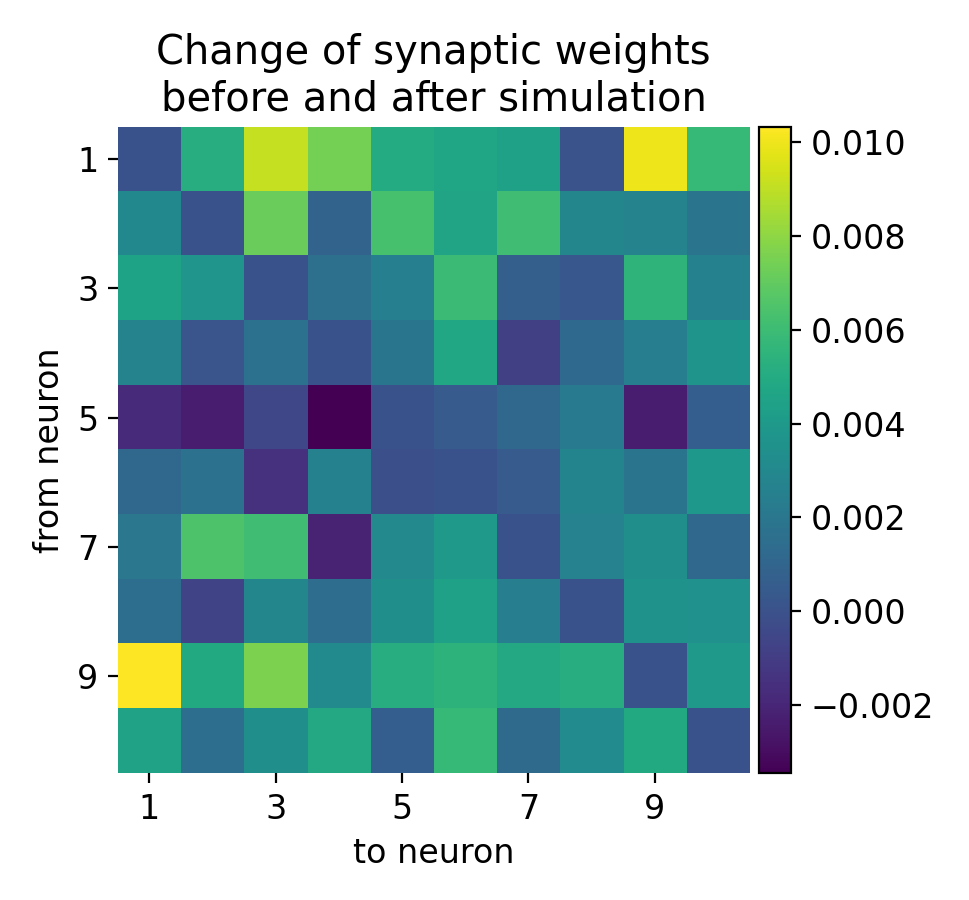
Synaptic weight changes in a large network with 10 excitatory and 3 inhibitory receiving inputs from 500 Poisson generators. The plot shows the change in synaptic weights before and after the simulation. Rows indicate presynaptic neurons and columns indicate postsynaptic neurons. The synaptic weights are normalized to the initial weight.

The resulting matrix of weight changes shows the plasticity effects in the network, with positive values indicating potentiation and negative values indicating depression. The matrix is not diagonal-symmetric because the Clopath rule allows for bidirectional plasticity, meaning the changes in synaptic weights are not necessarily the same in both directions between any two neurons. The Clopath rule modifies synaptic weights based on the precise timing of spikes between the presynaptic and postsynaptic neurons. If neuron $i$ fires before neuron $j$, the weight change from $i$ to $j$ can be different from the weight change from $j$ to $i$, leading to an asymmetric weight matrix. And each synaptic connection updates its weight independently. The weight from neuron $i$ to neuron $j$ ($w_{i\rightarrow j}$) and from neuron $j$ to neuron $i$ ($w_{j\rightarrow i}$) are updated based on their own specific spike timing and neuronal activity. This independent update mechanism naturally leads to non-symmetric changes.

In biological neural networks, synaptic plasticity is inherently direction-dependent. The synaptic strength from one neuron to another can be modulated differently compared to the reverse direction, reflecting the biological processes of learning and memory encoding. The LTP and LTD processes depend on the relative timing of pre- and postsynaptic spikes. The temporal asymmetry in spike timing (e.g., pre-before-post vs. post-before-pre) results in different synaptic modifications for each direction.

Thus, the lack of diagonal symmetry in the weight change matrix is a direct result of the nature of the Clopath rule, which inherently supports bidirectional, independent, and asymmetric synaptic weight updates. This property allows for more complex and realistic modeling of synaptic plasticity, capturing the nuanced and direction-specific nature of biological synapses.

Conclusion

The Clopath rule is not just another STDP curve. It is a voltage-based plasticity model that explicitly links synaptic change to the postsynaptic depolarization state. This makes it far more suitable than simple pair-based STDP rules for modeling experiments in which firing rate, subthreshold voltage, and repeated spike pairing all influence the direction and magnitude of synaptic plasticity.

I think, its main strength lies in the combination of mechanistic interpretability and computational simplicity. The rule remains compact enough for large network simulations, yet rich enough to capture important biological features such as voltage dependence, frequency dependence, and homeostatic stabilization. For this reason, it has become a standard choice whenever synaptic plasticity is meant to depend on more than spike timing alone.

The complete code used in this blog post is available in this Github repositoryꜛ. The spike pairing and recurrent network examples can be adapted easily to explore how voltage-based plasticity shapes synaptic organization under different input regimes.

The complete code used in this blog post is available in this Github repositoryꜛ (clopath_spike_pairing.py and clopath_bidirectional_connections.py). Feel free to modify and expand upon it, and share your insights.

References

• C. Clopath, L. Büsing, E. Vasilaki, Wulfram Gerstner, Connectivity reflects coding: a model of voltage-based STDP with homeostasis, 2010, Nat Neurosci, 13(3), 344-352. doi: 10.1038/nn.2479ꜛ
• Claudia Clopath, Wulfram Gerstner, Voltage and spike timing interact in STDP - a unified model, 2010, Frontiers in Synaptic Neuroscience, Vol. n/a, Issue n/a, pages n/a, doi: 10.3389/fnsyn.2010.00025
• Voltage-based STDP synapse (Clopath et al. 2010) on ModelDBꜛ
• Wulfram Gerstner, Werner M. Kistler, Richard Naud, and Liam Paninski, Chapter 19 Synaptic Plasticity and Learning Neuronal Dynamics: From Single Neurons to Networks and Models of Cognition, 2014, Cambridge University Press, ISBN: 978-1-107-06083-8, free online versionꜛ
• Jesper Sjöström, Wulfram Gerstner, Spike-timing dependent plasticity, 2010, Scholarpedia, 5(2):1362, doi: 10.4249/scholarpedia.1362ꜛ
• NEST’s tutorial “Clopath Rule: Spike pairing experiment”ꜛ
• NEST’s tutorial “Clopath Rule: Bidirectional connections”ꜛ
• NEST’s aeif_psc_delta_clopath model descriptionꜛ
• NEST’s clopath_synapse descriptionꜛ