Sparse component analysis: Finding separable computations in neural population activity

This coming Monday I will present a recent Neuron paper by Andrew J. Zimnik, Xinyue An, K. Cora Ames, and colleagues in our journal club: “Sparse component analysis: A method that uncovers separable computations within neural population activity” (doi:10.1016/j.neuron.2026.05.022ꜛ). I have been preparing the slides for that discussion, but the paper is interesting enough that I wanted to write down a more detailed version here.

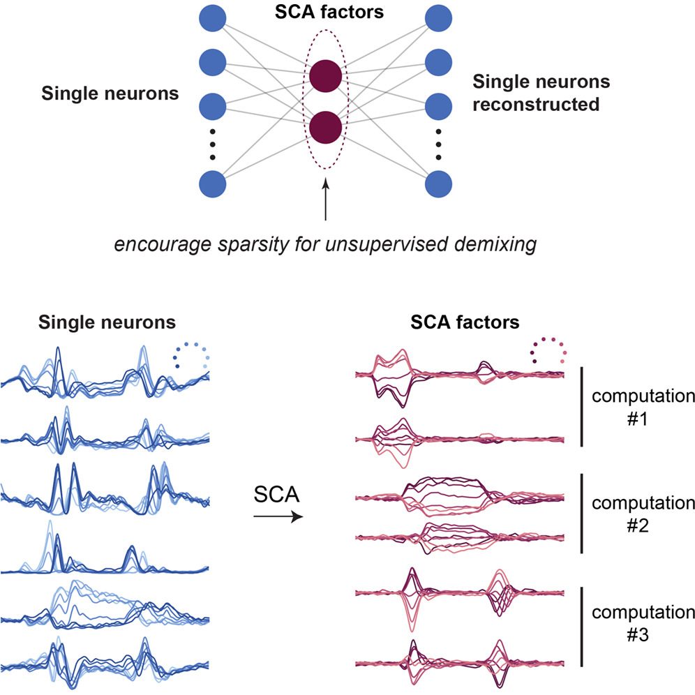Graphical abstract of Zimnik et al. (2026). Sparse component analysis (SCA) is an unsupervised dimensionality reduction method that, unlike PCA, does not only seek a low-dimensional reconstruction of neural population activity, but encourages latent factors to be temporally sparse and therefore more aligned with separable computations. In this post, we walk through the maths and main results behind this idea. Source: Zimnik et al. (2026), Neuron / Cell Press, 10.1016/j.neuron.2026.05.022ꜛ. © 2026 The Authors. Published by Elsevier Inc. Licensed under CC BY-NC-ND 4.0.

The central idea is simple, but powerful. Neural population activity is often low-dimensional, yet the axes returned by common dimensionality reduction methods are not necessarily the axes we would like to interpret biologically. Principal component analysis (PCA), for example, finds directions that explain variance. That is a statistically natural goal, but it is not the same as finding separate computations. Zimnik et al. propose sparse component analysis (SCA), an unsupervised method that keeps the reconstruction logic of dimensionality reduction but adds a biologically motivated preference: If distinct computations are used flexibly, they should often be non-synchronous, and therefore there should exist a latent basis in which each factor is active only during part of the task.

In this post, we will first describe the problem and build the mathematical framework from PCA to SCA, then we discuss the main results figure by figure, and finally we critically discuss the method and its limitations.

Problem statement

In Computational Neuroscience, we often want to understand how neural populations implement computations. A common approach is to record from many neurons simultaneously and then use dimensionality reduction to find a small number of latent factors that summarize the population activity. The idea behind this is that population activity lives in a lower-dimensional space than the number of recorded neurons. If we record $N$ neurons over $T$ time points, we, for instance can arrange the data in a matrix

\[X \in \mathbb{R}^{T \times N},\]

where each row is one time point and each column is one neuron. The usual dimensionality reduction goal is to find a small number $K \ll N$ of latent factors

\[Z \in \mathbb{R}^{T \times K}\]

that summarize the structure in $X$.

The problem is not merely dimensionality. The harder problem is, however, interpretability.

In a motor task, for instance, the same neuron may be active during preparation, movement execution, posture maintenance, and return movement. It may change its tuning across epochs. It may not cleanly belong to one functional class. At the level of single neurons, the population looks mixed. However, the population as a whole may still contain distinct computational processes: Preparation may occupy one set of dimensions, execution another, posture another, and stopping another. This creates a mismatch between two questions:

1. Which low-dimensional subspace reconstructs the data well?
2. Which low-dimensional axes correspond to separable computations?

PCA is very good at the first question. SCA is designed to address the second question without requiring task labels or manually defined epochs.

The key assumption is compositional flexibility. If a system can reuse computations in different orders, durations, or combinations, then the corresponding latent factors should not always be active together. Preparation can precede execution, overlap with it, be extended, shortened, cancelled, or repeated. This non-synchrony implies that the correct latent axes may be relatively sparse in time. SCA formalizes that intuition.

Mathematical framework

To approach the problem mathematically, we first review PCA and then describe how SCA modifies it.

Assume $X$ has been centered across time. PCA seeks a rank-$K$ approximation

\[\hat{X} = ZV,\]

where

• $X \in \mathbb{R}^{T \times N}$ is the neural data matrix,
• $T$ is the number of time points, possibly concatenated across conditions,
• $N$ is the number of neurons or units,
• $K$ is the number of latent dimensions,
• $Z \in \mathbb{R}^{T \times K}$ contains the low-dimensional latent factors,
• $V \in \mathbb{R}^{K \times N}$ maps latent factors back into neural space.

One way to write PCA is as a reconstruction problem:

\[\begin{align*} &\min_{Z,V} \|X - ZV\|_F^2 \quad \text{subject to} \\ & \text{orthonormality constraints on } V. \end{align*}\]

Here $|\cdot|_F$ is the Frobenius norm, i.e., the square root of the sum of squared matrix entries. In PCA, the solution can be obtained by singular value decomposition:

\[X = P \Sigma Q^\top.\]

Here $P$ contains the left singular vectors, $Q$ contains the right singular vectors, and $\Sigma$ is a diagonal matrix of singular values. The singular values quantify how much variance is captured along the corresponding singular-vector directions.

The first $K$ right singular vectors in $Q_K$ define the principal axes, and the scores are

\[Z_{\text{PCA}} = X Q_K = P_K \Sigma_K.\]

The rank-$K$ PCA reconstruction is

\[\hat{X}_{\text{PCA}} = Z_{\text{PCA}} Q_K^\top.\]

PCA has an optimality guarantee: Among all rank-$K$ linear reconstructions, it minimizes squared reconstruction error. Equivalently, it captures the maximum possible variance for $K$ orthogonal dimensions.

But this is also the limitation. PCA selects axes based on variance, not on biological separability. If two true latent processes are both active at different times but are mixed by a rotation, PCA may choose axes that combine them because this concentrates variance. Both PCA factors can then be active during both process windows. Such factors reconstruct the data well, but they are less interpretable.

The rotation problem

Suppose PCA has correctly found the two-dimensional subspace containing two true processes. Even then, the basis inside that subspace may be wrong.

Let $R \in \mathbb{R}^{K \times K}$ be an orthogonal rotation, so

\[R^\top R = RR^\top = I.\]

$I$ is the identity matrix. If we rotate the latent variables and counter-rotate the decoder,

\[Z' = ZR, \quad V' = R^\top V,\]

then the reconstruction is unchanged:

\[Z'V' = (ZR)(R^\top V) = ZV.\]

This is the core geometric fact behind the intuition of SCA. A whole family of bases can reconstruct the same data equally well. PCA chooses one based on variance. SCA asks whether another basis in the same or similar subspace is more sparse and therefore more interpretable.

For a minimal example, imagine two latent factors that never overlap:

\[z(t) = \begin{cases} (1,0) & \text{during process 1},\\ (0,1) & \text{during process 2}. \end{cases}\]

At either time point, the L1 norm is

\[\|z(t)\|_1 = |z_1(t)| + |z_2(t)| = 1.\]

Now rotate the basis by $45^\circ$. The point $(1,0)$ becomes

\[\left(\frac{\sqrt{2}}{2}, -\frac{\sqrt{2}}{2}\right),\]

with L1 norm

\[\left|\frac{\sqrt{2}}{2}\right| + \left|-\frac{\sqrt{2}}{2}\right| = \sqrt{2}.\]

The rotated basis reconstructs the same neural activity, but it is less sparse: Both factors are active when only one ground-truth process was active. This is the mathematical intuition behind the statement that non-synchronous computations are sparser in their correct basis than in a mixed basis.

From PCA to SCA

Zimnik et al. implement SCA as a linear autoencoder with three objectives:

1. reconstruct the original neural activity,
2. make the latent factor activity sparse,
3. encourage decoder directions to be orthonormal.

In a compact form, the linear SCA objective is

\[\begin{align*} \arg\min_{U,V,b_u,b_v} & \left\|W\left[X - \left((XU + b_u)V + b_v\right)\right]\right\|_F^2 \\ & + \lambda_{\text{sparse}} \|XU + b_u\|_1 \\ & + \lambda_{\text{orth}} \|VV^\top - I\|_F^2. \end{align*}\]

with:

• $X \in \mathbb{R}^{T \times N}$: neural activity,
• $U \in \mathbb{R}^{N \times K}$: encoder weights from neurons to latent factors,
• $b_u \in \mathbb{R}^{1 \times K}$: encoder offset,
• $Z = XU + b_u \in \mathbb{R}^{T \times K}$: latent factor activity,
• $V \in \mathbb{R}^{K \times N}$: decoder weights from latent factors back to neurons,
• $b_v \in \mathbb{R}^{1 \times N}$: decoder offset,
• $W \in \mathbb{R}^{T \times T}$: optional diagonal sample-weighting matrix,
• $\lambda_{\text{sparse}}$: strength of the sparsity penalty,
• $\lambda_{\text{orth}}$: strength of the orthogonality penalty,
• $I$: the $K \times K$ identity matrix.

The first term,

\[\left\|W\left[X - \left((XU + b_u)V + b_v\right)\right]\right\|_F^2,\]

is the reconstruction loss. It asks the latent factors to explain the neural population activity. The weighting matrix $W$ is useful because neural activity may be much stronger during some epochs than others. Without weighting, a method may prioritize high-amplitude movement execution and underfit lower-amplitude preparation.

The second term,

\[\lambda_{\text{sparse}} \|XU + b_u\|_1,\]

is the defining SCA term. Importantly, SCA encourages sparse factor activity, not sparse loadings. This distinguishes it from sparse PCA. Sparse PCA asks each factor to involve only a subset of neurons. SCA asks each factor to be active only during restricted parts of the task. This is exactly what one wants if a computation is transient, flexible, or reused compositionally.

The third term,

\[\lambda_{\text{orth}} \|VV^\top - I\|_F^2,\]

encourages decoder directions to be orthogonal. Without this term, an optimization procedure could split one true process into multiple nearly collinear sparse factors. That would look sparse but would not represent distinct computations. Orthogonality is therefore not just a technical detail; it is a safeguard against over-sparsification.

The authors also constrain each row of $V$ to have unit norm. This prevents a trivial scaling solution in which $Z$ becomes arbitrarily small and $V$ becomes arbitrarily large. It also makes the magnitude of a factor more interpretable: A larger latent value corresponds to a larger effect on neural population activity.

What SCA does and does not assume

SCA does not know the task epochs. It does not know which time points are preparation, movement, posture, stopping, or mating motifs et cetera. It does not receive behavioral labels. It only sees population activity and optimizes the cost function above. The assumptions made for SCA are therefore broad but still real:

• distinct computations should correspond to distinct latent factors,
• those factors should often be non-synchronous,
• their mappings into neural activity should be close to orthogonal,
• the factors should still reconstruct the data well.

The last point is actually central: SCA is not merely searching for any sparse signal, it searches for sparse factors that still explain neural activity. If no sparse basis exists, forcing sparsity should increase reconstruction error, and the optimization should not strongly prefer it.

A simplified Python implementation

Zimnik et al. provide a full SCA implementation in their GitHub repositoryꜛ, from where you can easily install it with pip. However, for the purpose of the journal club, I wrote a simplified version that is easier to read and understand. It is not optimized for speed or stability, but it captures the core idea of SCA. You can find it in my GitHub repositoryꜛ.

The script creates a synthetic dataset with two partially overlapping latent processes, mixes them into heterogeneous single-neuron responses, runs PCA, and then performs a simple SCA-style rotation within the two-dimensional PCA subspace. This is not the full SCA algorithm from the paper, but a didactic approximation that isolates one key idea: If PCA has found the correct subspace, a sparsity objective can choose a more interpretable basis inside that subspace.

The generative structure is:

\[Z_{\text{true}} \in \mathbb{R}^{T \times 2},\]

with two non-synchronous processes. Neural activity is generated as

\[X = Z_{\text{true}} A L + \epsilon,\]

where

• $A \in \mathbb{R}^{2 \times 2}$ is a mixing rotation,
• $L \in \mathbb{R}^{2 \times N}$ maps latent processes into $N$ neurons,
• $\epsilon$ is Gaussian noise.

PCA then estimates

\[Z_{\text{PCA}} = X Q_2.\]

The simplified SCA-style step searches over two-dimensional rotations:

\[Z_\theta = Z_{\text{PCA}} R(\theta),\]

where

\[R(\theta) = \begin{bmatrix} \cos\theta & -\sin\theta \\ \sin\theta & \cos\theta \end{bmatrix}.\]

For each rotation angle $\theta$, the script computes

\[J(\theta) = \frac{1}{TK}\sum_{t=1}^{T}\sum_{k=1}^{K} |Z_{\theta,t,k}|.\]

The chosen rotation is

\[\theta^{\ast} = \arg\min_\theta J(\theta).\]

The key code looks like this:

def pca_factors(x: np.ndarray, n_components: int = 2) -> tuple[np.ndarray, np.ndarray]:
    """PCA scores and loadings from SVD, no scikit-learn required."""
    u, s, vt = np.linalg.svd(x, full_matrices=False)
    scores = u[:, :n_components] * s[:n_components]
    loadings = vt[:n_components]
    return scores, loadings

def rotation_matrix(theta: float) -> np.ndarray:
    return np.array([[np.cos(theta), -np.sin(theta)], [np.sin(theta), np.cos(theta)]], dtype=float,)

def sparse_orthogonal_rotation(
    z_pca: np.ndarray,
    n_grid: int = 720) -> tuple[np.ndarray, float, np.ndarray, np.ndarray]:
    """Find the 2D orthogonal rotation with minimal temporal L1 norm."""
    angles = np.linspace(0, np.pi, n_grid, endpoint=False)
    l1_values = np.empty_like(angles)
    for i, theta in enumerate(angles):
        rotated = z_pca @ rotation_matrix(theta)
        l1_values[i] = np.mean(np.abs(rotated))

    best_idx = int(np.argmin(l1_values))
    best_angle = float(angles[best_idx])
    return z_pca @ rotation_matrix(best_angle), best_angle, angles, l1_values

This intentionally leaves out several features of full SCA:

• it does not learn $U$ and $V$ jointly,
• it does not optimize a reconstruction plus sparsity plus orthogonality objective,
• it does not include sample weighting,
• it only works in the two-dimensional case,
• it assumes PCA has already found the correct subspace.

However, these simplifications are the actual core of the script, that let us see the geometry directly:

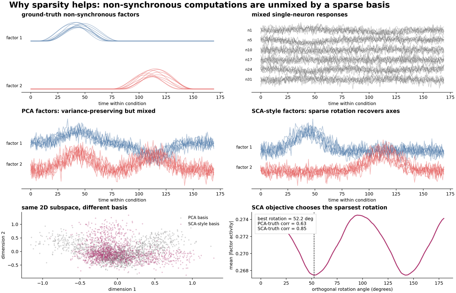Synthetic PCA-vs-SCA-style demonstration. The dataset contains two ground-truth latent processes, mixed single-neuron responses, PCA factors, SCA-style rotated factors, the shared two-dimensional state space, and the L1 objective across possible rotations. The code to reproduce this figure is available in my GitHub repositoryꜛ.

The upper-left panel shows the ground-truth latent processes. They are temporally flexible and partially overlapping. The upper-right panel shows example single-neuron responses. No neuron is a clean copy of one process; each neuron is a mixed linear combination plus noise.

The middle-left panel shows PCA factors. PCA finds the relevant two-dimensional subspace, but its axes are mixed. Both factors carry activity in both process windows. The middle-right panel shows the SCA-style rotated factors. The rotation does not change the subspace, but it aligns the axes more closely with the two ground-truth processes.

The lower-left panel is the geometric heart of the demo. The point cloud is the same population activity represented in two coordinate systems. PCA and SCA-style factors span the same two-dimensional plane. No information has been added. No reconstruction has been improved by magic. What changed is the basis inside the plane: PCA chooses axes according to variance; the SCA-style rotation chooses axes according to temporal sparsity.

The lower-right panel shows the objective $J(\theta)$ across rotation angles. The minimum marks the rotation with the smallest mean absolute factor activity. This rotation is favored because it concentrates activity into more localized temporal windows rather than spreading both processes across both axes. In this run, the mean absolute correlation with ground-truth factors improved from about 0.63 for PCA to about 0.85 for the SCA-style rotation.

Again, this is only a demonstration example. Full SCAꜛ solves the more general problem directly in the neural data (the official SCA repo also contains two neural datasets), but the intuition is the same: Among bases that reconstruct the population well, prefer the one in which latent activity is temporally sparse and decoder directions remain distinct.

Non-linear SCA

Zimnik et al. also develop a non-linear version of SCA. This is useful if the relationship between latent factors and neural activity is not well described by a purely linear decoder.

In non-linear SCA, an encoder network

\[f_{\theta_f}: \mathbb{R}^{N} \rightarrow \mathbb{R}^{K}\]

maps neural activity to latent factors

\[Z = f_{\theta_f}(X),\]

and a decoder network

\[g_{\theta_g}: \mathbb{R}^{K} \rightarrow \mathbb{R}^{N}\]

maps factors back to neural activity:

\[\hat{X} = g_{\theta_g}(Z) = g_{\theta_g}(f_{\theta_f}(X)).\]

The non-linear objective is

\[\begin{align*} \arg\min_{\theta_f,\theta_g} & \left\|W\left[X - g_{\theta_g}(f_{\theta_f}(X))\right]\right\|_F^2 \\ & + \lambda_{\text{sparse}} \|f_{\theta_f}(X)\|_1 \\ & + \lambda_{\text{orth}} \sum_i \|V_iV_i^\top - I\|_F^2. \end{align*}\]

Here $V_i$ denotes the weight matrix of decoder layer $i$. Orthonormality is strictly defined for linear maps, so in the non-linear case this term is best interpreted as encouraging different latent factors to map into neural activity through distinct decoder directions. In Zimnik et al.’s implementation, both encoder and decoder use a single hidden layer with a $\tanh$ non-linearity.

The non-linear extension matters for reconstruction. In the unimanual cycling data example Zimnik et al. discuss in the paper, non-linear SCA reconstructs held-out activity better than linear SCA at the same number of dimensions. But the striking result is that the dominant factor categories remain similar: Preparation, steady-state execution, posture, and stopping. That makes the non-linear result a useful sanity check. The separable computational structure is thus not merely an artifact of the linear method.

Results

In the following, we walk through the main results of the paper figure by figure. I will not show every panel, but I will highlight the most important ones and discuss their interpretation.

The core intuition (Figure 1)

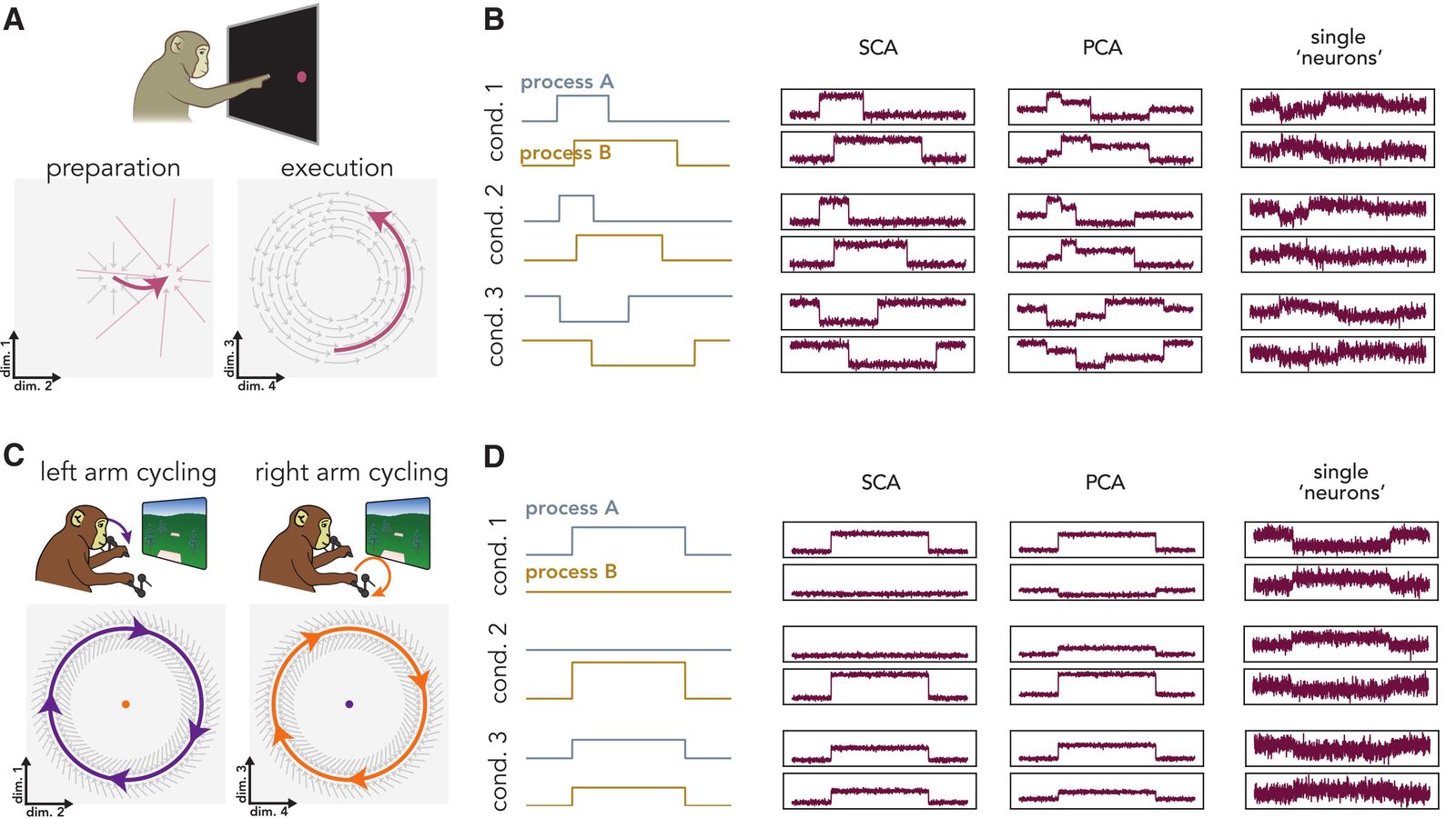Figure 1A-D from Zimnik et al. These panels motivate two forms of non-synchronous latent structure: Preparation versus execution during reaching (A, B), and left-arm versus right-arm factors during cycling (C, D). In both simulations, SCA recovers the ground-truth processes more cleanly than PCA (B, D), despite mixed single-neuron responses. Source: Zimnik et al. (2026), Neuron / Cell Press, 10.1016/j.neuron.2026.05.022ꜛ. © 2026 The Authors. Published by Elsevier Inc. Licensed under CC BY-NC-ND 4.0.

Figure 1A uses reaching as the canonical example. Preparation and execution are not merely two time periods; they are associated with different population-level dynamics. Preparatory activity can be relatively stable, while execution-related activity can evolve through a different dynamical pattern. Figure 1B turns this into a synthetic test. Two ground-truth processes vary in timing and duration across conditions. They are mixed into simulated neurons (in principle, in our custom Python script we adopted the same approach). The single neurons look noisy and mixed. PCA recovers factors that still mix the two processes, whereas SCA recovers the underlying process time courses more clearly.

Figure 1C gives a complementary example: Left-arm and right-arm cycling. Left-arm factors should be active during left-arm movement and quiet during right-arm movement; right-arm factors should show the opposite pattern. During bimanual movement, both sets can be co-active. That is compositional reuse. Figure 1D shows again the corresponding simulation. Also here, SCA benefits from the fact that the two processes can occur alone or together. This non-synchrony creates a sparse basis that PCA is not designed to find.

The paper’s remaining Figure 1 panels H-I formalize the geometry and limitations. I am not showing them here, but their message is important to mention: Sparsity recovers the correct basis when factors are sufficiently non-overlapping. If two processes overlap too strongly, the sparsest rotation may instead capture their common activity and their difference. That is not necessarily a failure. It may mean that the experiment does not provide enough temporal flexibility to justify separating the processes.

A reaching experiment: From mixed PCA factors to interpretable SCA factors (Figure 2)

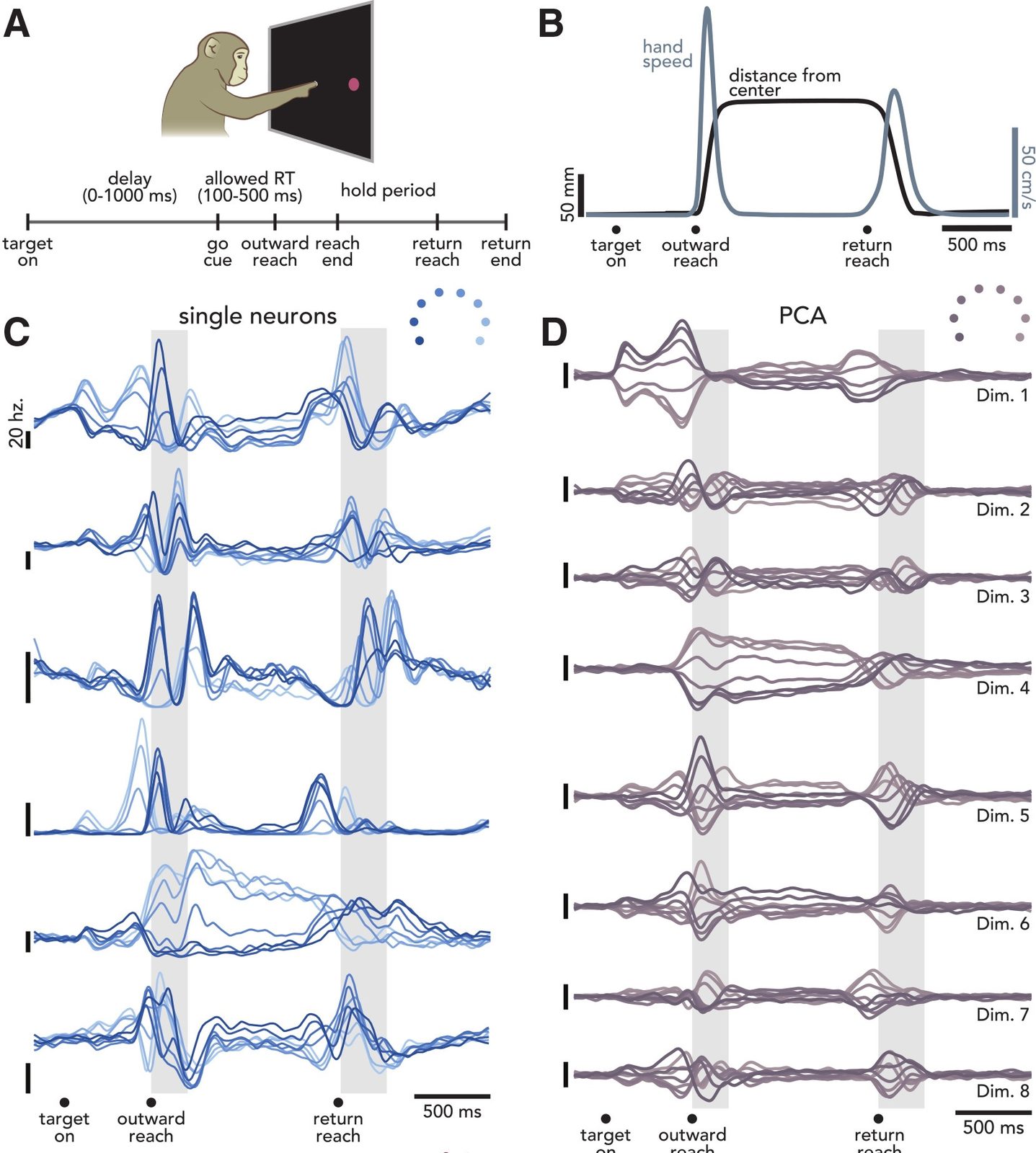Figure 2A-D. Center-out reaching task, behavior, example neurons, and PCA factors. The single-neuron responses and PCA factors mix preparation, execution, posture, and return-related activity. Source: Zimnik et al. (2026), Neuron / Cell Press, 10.1016/j.neuron.2026.05.022ꜛ. © 2026 The Authors. Published by Elsevier Inc. Licensed under CC BY-NC-ND 4.0.

Paper Figure 2 demonstrates SCA applied to the first real dataset. The task is a center-out reaching experiment. Monkeys hold at a central touch point, see a target, wait through a delay, reach outward after the go cue, hold the new posture, and then return to the start position. The dataset contains recordings from motor cortex neurons during this task. The relevant hypothesis is already well established in the motor cortex literature: Preparation and execution occupy distinct population dimensions. More recent work also suggests posture-related factors during holding. The question is whether an unsupervised method can recover these categories without being told the epoch boundaries.

Panels A and B show the task and behavior. Panel C shows example neurons. These neurons are not neatly separated into “preparatory neuron”, “movement neuron”, or “posture neuron”. A neuron can be active across several periods, and its tuning can change across epochs. Panel D shows the corresponding top PCA factors. They are also mixed. Some factors hint at particular epochs, but many remain active across much of the trial. This is the classic PCA problem: The subspace is useful, but the basis is not biologically clean.

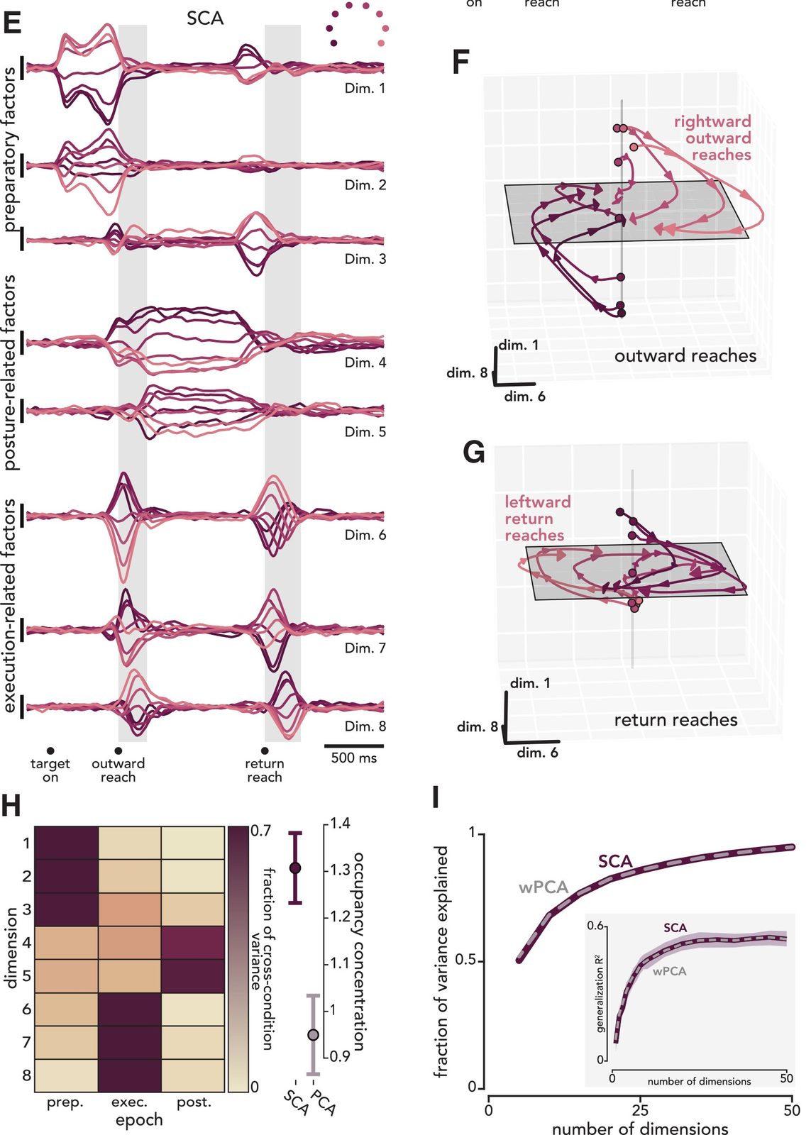Figure 2E-I. SCA identifies factors primarily active during preparation, execution, or posture. It preserves reconstruction performance relative to weighted PCA while increasing epoch-specific occupancy. Source: Zimnik et al. (2026), Neuron / Cell Press, 10.1016/j.neuron.2026.05.022ꜛ. © 2026 The Authors. Published by Elsevier Inc. Licensed under CC BY-NC-ND 4.0.

Panel E then shows the SCA factors and is probably the most important panel in the paper. Here, eight SCA factors now fall into interpretable classes. Dimensions 1-3 are mainly active before movement and are interpreted as “preparatory” factors. Dimensions 6-8 are active around movement and are interpreted as “execution-related” factors. Dimensions 4-5 remain active during the hold period and are interpreted as “posture-related” factors. This interpretation is strengthened by the return reach. Before the return reach, posture-related activity drops back toward baseline, preparatory activity reemerges, and execution-related activity rises around movement. The same functional sequence appears again, but in reverse behavioral context.

In addition to this, panels F and G show the underlying geometry. Activity rotates from a preparatory dimension into an execution-related plane. This reproduces and extends a known dynamical systems view of motor cortex: Preparation sets an initial condition, and execution unfolds through movement-related dynamics.

Panel H offers another perspective and quantifies factor concentration across epochs. SCA factors tend to have most of their occupancy in one epoch, whereas weighted PCA factors are more spread out. Panel I is equally important as it addresses the most obvious concern: Is SCA interpretable only because it sacrifices reconstruction? The answer: It does not. SCA and weighted PCA explain nearly identical neural variance and generalize similarly to held-out neurons and time points.

The final lesson from this experiment is in my view not that PCA is inherently wrong. PCA solves a different problem. It finds the subspace that explains variance. SCA, on the other hand, finds a basis inside that subspace that is more interpretable. The two methods are thus complementary while SCA additionally provides a biologically interpretable basis.

Supervision helps only when the labels match the computation (Figure 3)

In Figure 3 (not shown here), the authors compare SCA, by default unsupervised, with supervised approaches. They show that a properly supervised method, given accurate epochs for preparation, execution, and posture, performs very well, which is expected. If we already know the correct computational categories and their timing, supervision can isolate them. The more interesting comparison is with imperfect supervision. A naively supervised approach that knows only a coarse separation between preparation and movement, but not posture, mixes execution and posture-related factors. Demixed PCA also demixes according to the labels it is given, but those labels do not necessarily correspond to the computational processes of interest. This co-investigation adds a valuable perspective: SCA is not a replacement for supervision, but the latter is not automatically more “biological”. It is only as good as the labels. SCA is valuable precisely when the correct labels or epoch boundaries are unknown.

The second experiment: Unimanual cycling (Figure 4)

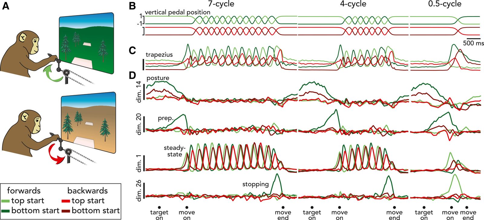Figure 4. SCA applied to unimanual cycling. (A) Task schematic: Monkeys moved a handheld pedal forward or backward along a virtual track, starting either near the top or bottom of the cycle and stopping at targets placed at different distances. (B) Vertical pedal position for example conditions, showing the cyclic behavioral structure and the different movement durations. (C) Example EMG activity, illustrating that muscle activity depends on cycling direction and start/end posture. (D) Four representative SCA factors corresponding to posture, preparation, steady-state execution, and stopping. The stopping factor becomes active shortly before movement termination, suggesting a separable process related to ending the ongoing movement. Source: Zimnik et al. (2026), Neuron / Cell Press, 10.1016/j.neuron.2026.05.022ꜛ. © 2026 The Authors. Published by Elsevier Inc. Licensed under CC BY-NC-ND 4.0.

Figure 4 moves from brief, externally cued reaches to extended cyclic movements that unfold over several seconds. The task structure illustrated in panel A is much more complex (or richer) than in the previous reaching experiment from Figure 2: Monkeys cycle a handheld pedal forward or backward through a virtual track, beginning from either a top or bottom starting position and stopping at targets placed at different distances. This design creates a useful test case for SCA, because the task contains several candidate computations whose timing can vary: Maintaining an initial posture, preparing a movement, producing rhythmic cycling, and terminating the movement.

In panel B, the behavioral scaffold of the experiment is shown. The vertical pedal position oscillates during cycling, and the number of cycles changes across conditions. Four-cycle and seven-cycle movements contain an extended steady-state phase, whereas half-cycle movements are much shorter. This is important because it allows to ask whether longer movements are built by stretching or repeating a shared execution-related process, rather than by recruiting entirely different factors for each movement duration. Panel C provides a muscle-level reference ti this. The example EMG activity depends on cycling direction and on the start or end position of the arm. This is important for interpreting the latent factors in panel D: If a factor is posture-related, preparatory, or stopping-related, its condition dependence should make sense with respect to the muscle patterns and the behavioral state. And here, SCA identifies four interpretable factor classes. The “posture” factor is active between movements and reflects the maintained arm configuration. The “preparatory” factor becomes active before movement onset and depends on the upcoming movement. The “steady-state execution” factor is rhythmic during ongoing cycling and tracks the repeated movement structure. The “stopping” factor becomes active shortly before movement termination.

The stopping factor is the most interesting new element in this study as it was not a standard category that one would necessarily define in advance. Yet it emerges naturally from the unsupervised SCA objective. Its timing, shortly before the movement ends, and its dependence on final position and cycling direction make several interpretations plausible: It may reflect preparation to stop, a stopping-specific execution process, sensory-feedback-related control near the target, or some combination of these. The cautious interpretation is therefore not simply “SCA found stopping”, but rather: SCA found a separable latent factor whose timing and tuning are consistent with a stopping-related computation.

The compositional point follows directly from comparing panels B and D. Seven-cycle and four-cycle movements use similar factor categories, but the steady-state execution period is longer for the longer movement. Half-cycle movements appear to reuse much of the same structure, though with a truncated execution phase. Thus, SCA does not merely classify activity into epochs; it suggests that extended actions can be assembled from reusable latent components whose duration and ordering change with the behavioral demand.

The authors are appropriately careful not to overinterpret this result. Calling a factor “stopping” is a hypothesis, not a proof. But that is precisely why this figure is so valuable in ym view: SCA turns a complex population response into a set of candidate computations that can be tested with further analyses or experiments.

Bimanual cycling: Compositional reuse without simple addition (Figure 5)

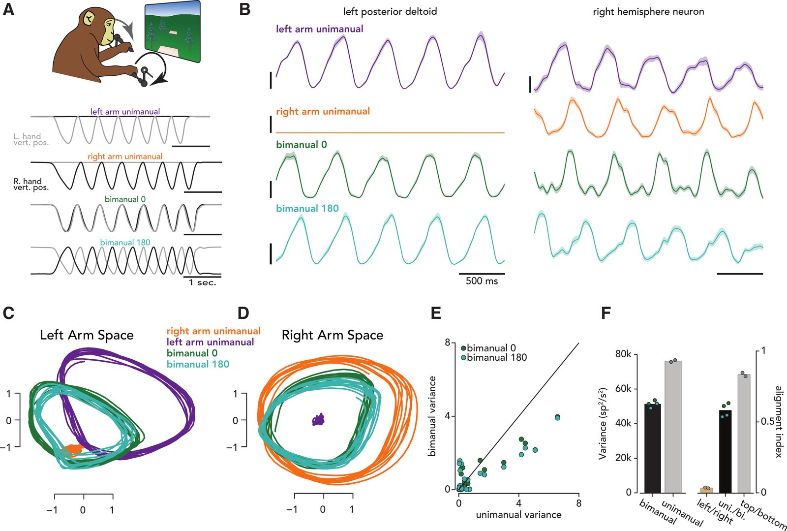Figure 5. SCA applied to bimanual cycling. (A) Task schematic and example hand-position traces for left-arm-only, right-arm-only, and bimanual cycling, with the two arms either in phase or out of phase. (B) Example EMG and single-neuron activity: Muscle activity is largely arm-specific, whereas a motor cortex neuron can respond during movements of either arm. (C-D) SCA identifies left-arm and right-arm factors. These factors are active during the corresponding unimanual movement and are reused during bimanual movement. (E) Factor-wise variance during bimanual movement is often smaller than predicted by simple superposition of the two unimanual conditions. (F) Population-level analyses show the same pattern: Bimanual activity partially reuses unimanual subspaces, but not as a perfect linear sum. Source: Zimnik et al. (2026), Neuron / Cell Press, 10.1016/j.neuron.2026.05.022ꜛ. © 2026 The Authors. Published by Elsevier Inc. Licensed under CC BY-NC-ND 4.0.

Figure 5 asks whether bimanual movement is built by reusing latent factors that are already present during unimanual movement. Panel A lays out the task: Monkeys cycle with the left arm alone, the right arm alone, or both arms together. In the bimanual conditions, the two arms move either in phase or with a 180-degree phase offset. This design separates two possibilities: Bimanual control could recruit the same left- and right-arm factors used during unimanual movement, or it could rely on a distinct bimanual control regime.

Panel B shows why the population-level analysis is necessary. The EMG example on the left is largely arm-specific: Left-arm muscle activity mainly reflects what the left arm is doing. The cortical neuron on the right, however, is active during movements of either arm. At the level of single neurons, the representation therefore looks mixed. This is exactly the kind of situation where SCA becomes useful: A neuron may participate in several latent factors, even if those factors are separable at the population level.

Panels C and D then show the central SCA result. Panel C plots two left-arm factors, which have large trajectories during left-arm-only cycling, very small trajectories during right-arm-only cycling, and large trajectories again during bimanual cycling. Panel D shows the complementary pattern for right-arm factors: They are active during right-arm-only cycling, largely quiet during left-arm-only cycling, and active again when both arms move. This is a clear example of compositional reuse. Bimanual movement appears to recruit both the left-arm and right-arm factor sets.

The result is not simply that the cortex contains an abstract “cycling” factor shared by both arms. If that were the case, one would expect substantial overlap between left-arm-only and right-arm-only conditions. Instead, panels C and D show that the left- and right-arm factors are mostly distinct during unimanual cycling. They become co-active during bimanual cycling. Bimanual control is compositional because it combines separable arm-specific factors, not because the same factor is used for every cycling movement.

Panels E and F then test whether this composition is just linear addition. Panel E compares, for individual SCA factors, the variance observed during bimanual cycling with the variance predicted by summing the corresponding unimanual variances. If bimanual activity were a simple superposition of left-arm and right-arm activity, the points should fall near the identity line. Instead, many factors show less bimanual variance than predicted. In other words, the bimanual trajectories reuse unimanual factors, but their amplitudes are compressed or otherwise modified. Panel F makes the same point at the population level. The left plot shows that total neural variance during bimanual cycling is smaller than expected under simple superposition. The right plot shows subspace alignment. Alignment between left-arm-only and right-arm-only activity is close to zero, consistent with distinct arm-specific factor sets. Alignment between bimanual and unimanual activity is high, consistent with reuse. But it is not perfect, consistent with bimanual-specific modifications and with the fact that SCA also identifies some factors active primarily during bimanual movement.

The interpretation is therefore nicely balanced: Motor cortex activity during bimanual cycling is not just a collection of contralateral single-arm signals, because individual neurons can be active during movements of either arm, but it is also not a perfect sum of two independent unimanual controllers. SCA reveals a compositional structure instead: Left-arm and right-arm factors are separable, reused together during bimanual movement, and modified by the demands of coordinating both arms.

Motif-related factors in C. elegans (Figure 6)

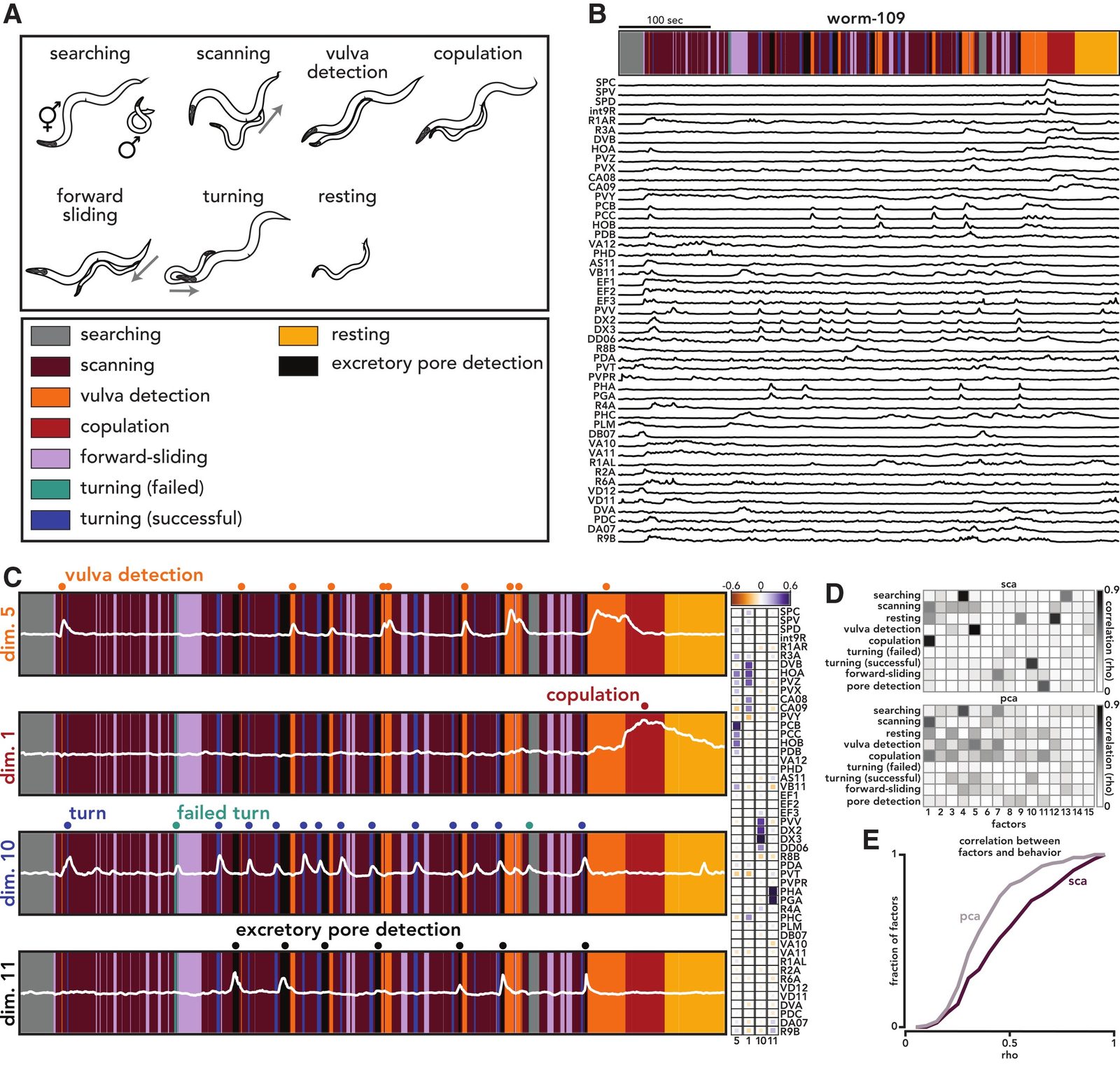Figure 6A-E. In single-trial calcium imaging from male C. elegans during mating, SCA identifies factors related to specific behavioral motifs and maps them onto identified neurons. Source: Zimnik et al. (2026), Neuron / Cell Press, 10.1016/j.neuron.2026.05.022ꜛ. © 2026 The Authors. Published by Elsevier Inc. Licensed under CC BY-NC-ND 4.0.

Zimnik et al. then move to a very different system: C. elegans. The worm has only 302 neurons, and they are identifiable across animals. This is in contrast to monkey motor cortex, where single neurons are often highly mixed and not identifiable across animals. In C. elegans, neurons can be more tightly linked to particular behaviors. Here, the data come from male worms during mating. Behavior is divided into motifs such as turning, vulva detection, copulation onset, and excretory pore detection (Panel A). SCA is applied separately to each worm, without using the behavioral labels.

Panel B shows an ethogram and calcium activity for 49 neurons during one mating bout. Panel C shows example SCA factors. These factors are closely tied to behavioral motifs: One around vulva detection, one around copulation onset, one around turning, and one around excretory pore detection. The loadings are especially satisfying because they map onto known neuron functions. For example, a vulva-detection factor loads onto neurons known to contribute to vulva detection; a turning-related factor loads strongly onto PVV, a neuron implicated in turning behavior.

Panels D and E quantify this relationship. For each factor, the correlation with behavioral motifs is computed. SCA factors tend to correlate more strongly with a single best motif than weighted PCA factors do. The paper reports an average best-motif correlation of about 0.47 for SCA versus 0.37 for weighted PCA, with $p \lt 0.001$.

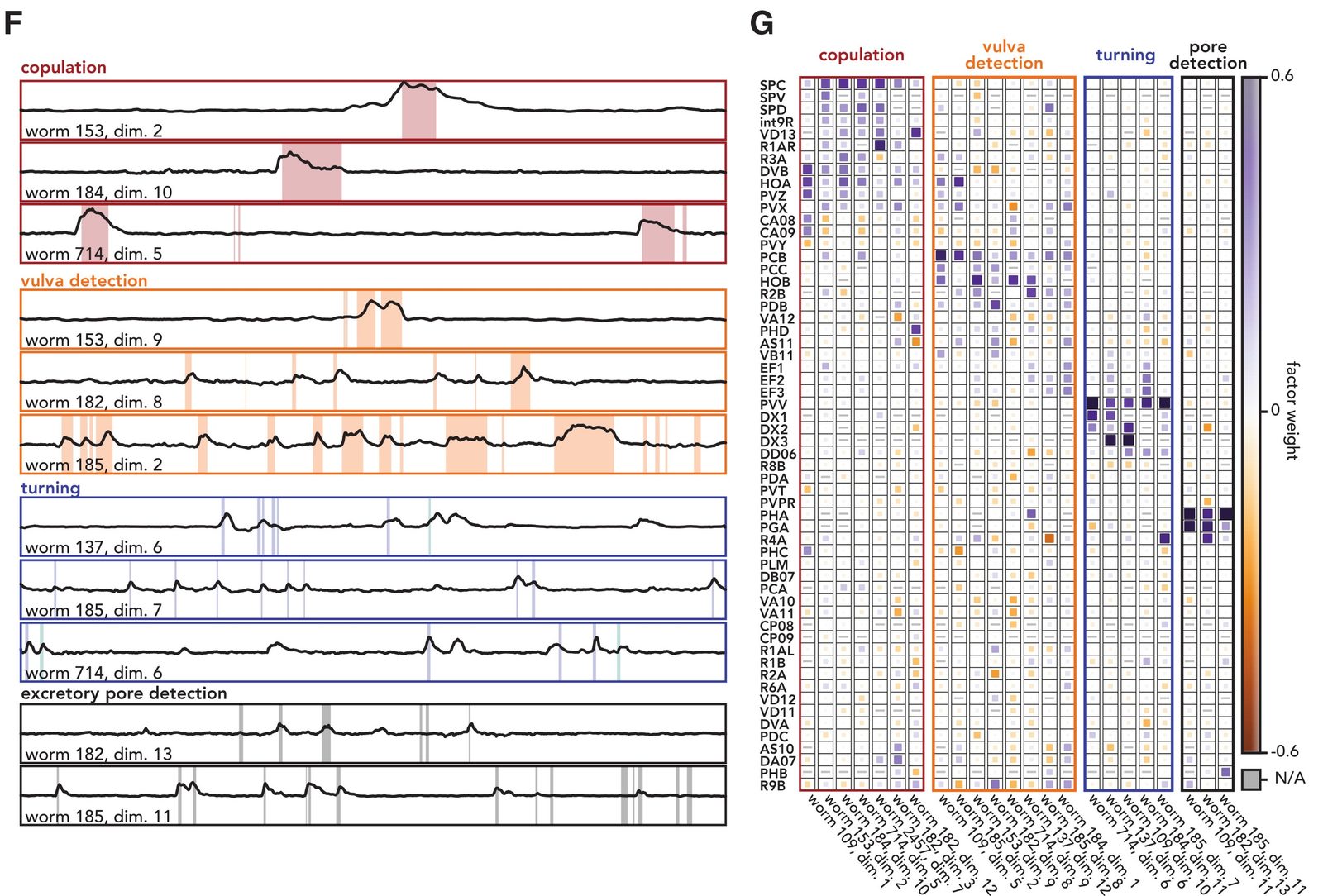Figure 6F-G. Motif-related SCA factors and loadings are partially reproducible across worms, despite incomplete overlap in recorded neurons. Source: Zimnik et al. (2026), Neuron / Cell Press, 10.1016/j.neuron.2026.05.022ꜛ. © 2026 The Authors. Published by Elsevier Inc. Licensed under CC BY-NC-ND 4.0.

Panels F and G extend the so-far findings and address reproducibility across an entire cohort of animals. And indeed, similar motif-related factors appear in different worms. The corresponding loadings also show biologically meaningful consistency: Copulation-related factors tend to weight neurons such as SPC, SPD, and HOA; turning-related factors tend to weight PVV. This is important because it shows that SCA is not only producing interpretable axes within one dataset. In this system, where neurons are identifiable, some of the factor-neuron relationships generalize across animals.

Compositionality in a multitask RNN (Figure 7)

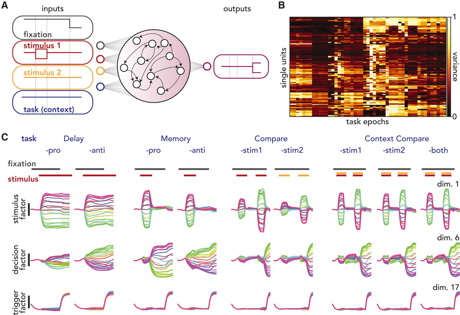Figure 7. In a multitask recurrent neural network, SCA identifies factors corresponding to task-relevant stimulus representation, internal decision variables, and output timing. Source: Zimnik et al. (2026), Neuron / Cell Press, 10.1016/j.neuron.2026.05.022ꜛ. © 2026 The Authors. Published by Elsevier Inc. Licensed under CC BY-NC-ND 4.0.

The authors then turn to a synthetic test case: A recurrent neural network trained on multiple cognitive tasks. This is a valuable add-on-experiment because the network is a system in which compositional computational structure is expected from previous work, which adds a strong conceptual test of SCA. The network receives stimulus inputs in two channels, context inputs specifying the task, and produces a two-dimensional directional output. Its dynamics can be written as

\[\tau \frac{dh}{dt} = -h(t) + F(W_{\text{rec}}h(t) + W_{\text{in}}u(t) + b_{\text{in}}),\] \[z(t) = W_{\text{out}}h(t) + b_{\text{out}},\]

where $h(t)$ is the recurrent state, $u(t)$ is the input, $F$ is a non-linear activation function, and $z(t)$ is the output. $\tau$ is the time constant of the recurrent dynamics, $W_{\text{rec}}$ is the recurrent weight matrix, $W_{\text{in}}$ is the input weight matrix, $W_{\text{out}}$ is the output weight matrix, and $b_{\text{in}}$ and $b_{\text{out}}$ are offset terms.

Panel B shows that individual units are active across many task epochs. At the unit level, the network looks mixed.

Panel C shows three SCA factors. One factor reflects the task-relevant stimulus, regardless of the input channel. Another reflects the internal decision: In pro and anti tasks, its ordering flips in a way that predicts the later response. A third factor resembles a condition-invariant trigger signal after the go cue. Thus, SCA recovers building blocks in a system where the computational structure is known to be compositional, but where individual units do not cleanly reveal that structure. This is a strong conceptual validation of the method.

Non-linear SCA improves reconstruction while preserving interpretability (Figure 8)

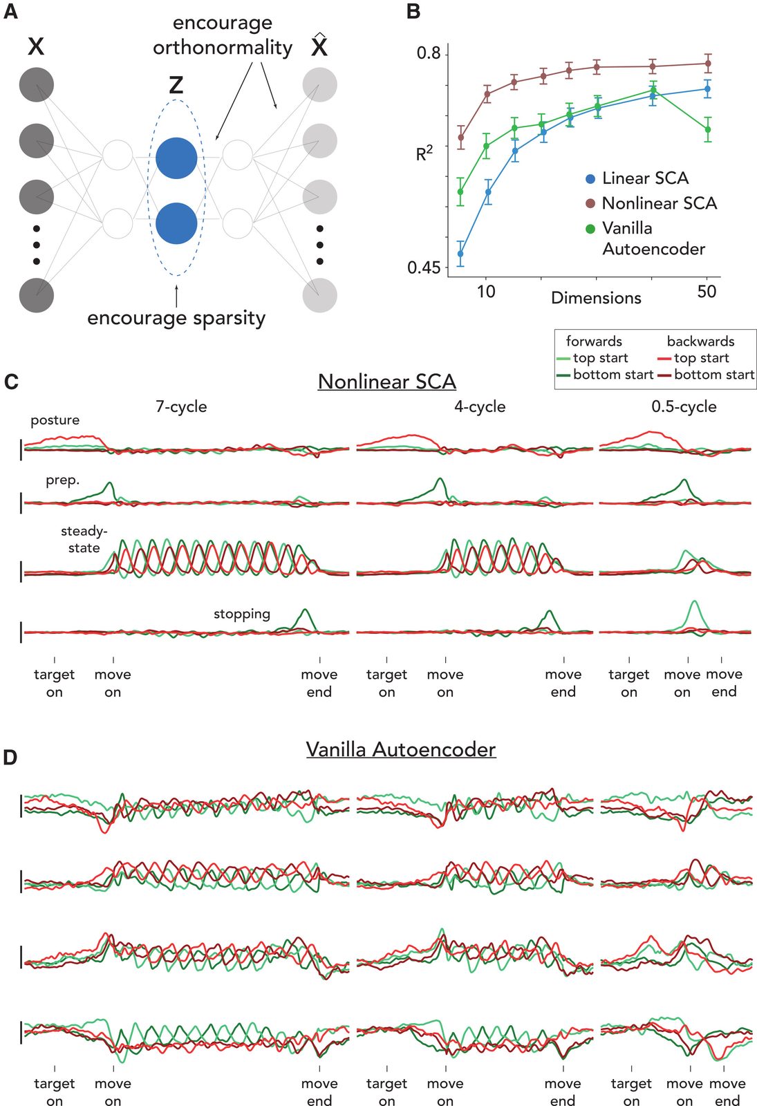Figure 8. Non-linear SCA reconstructs unimanual cycling data better than linear SCA at the same dimensionality, while preserving interpretable factor categories. A vanilla autoencoder reconstructs activity but yields more mixed factors. Source: Zimnik et al. (2026), Neuron / Cell Press, 10.1016/j.neuron.2026.05.022ꜛ. © 2026 The Authors. Published by Elsevier Inc. Licensed under CC BY-NC-ND 4.0.

In their last experiment, Zimnik et al. explore a non-linear extension of SCA. The motivation is that the relationship between latent factors and neural activity may not be well described by a purely linear decoder. Non-linear SCA uses an encoder network to map neural activity to latent factors and a decoder network to map factors back to neural activity. The objective includes terms for reconstruction error, sparsity of latent factors, and orthonormality of decoder weights. In particular, non-linear SCA, linear SCA, and a vanilla autoencoder are compared on the unimanual cycling dataset.

Panel A shows the non-linear architecture. The latent factors are still penalized for non-sparsity, and decoder weights are encouraged to be orthonormal. Panel B shows held-out reconstruction performance. Non-linear SCA achieves higher $R^2$ than linear SCA with fewer dimensions. This is expected if some neurons are non-linear functions of the underlying factors.

Panel C shows that non-linear SCA still finds interpretable factor categories: Posture, preparation, steady-state execution, and stopping. Panel D shows the control: A vanilla autoencoder without the sparsity and orthonormality terms can reconstruct activity, but its factors are mixed and less interpretable. Thus, reconstruction alone is not enough. A flexible autoencoder can fit the data but may not yield useful latent axes. SCA’s regularization terms act as an inductive bias toward separable computations.

Critical perspective

I like this paper because the method is conceptually aligned with a real neuroscientific question. It is not just “here is another dimensionality reduction algorithm”. It asks: If computations are flexibly composed, what should their latent factors look like? At the same time, the method should be interpreted carefully.

First, SCA does not name factors. The labels “preparation”, “execution”, “posture”, “stopping”, or “copulation” come from the scientist, not from the optimization. SCA provides candidate axes and temporal structure, but biological interpretation still requires domain knowledge, controls, and follow-up experiments.

Second, sparsity is a hypothesis. This hypothesis is plausible for many flexible behaviors, but it is not universally guaranteed. If two processes are always co-active, SCA may not separate them: When the overlap becomes too large, the sparsest basis is no longer the original two-factor basis (see core intuition experiment in their Figure 1). This is a limitation, but also a useful conceptual constraint: If an experiment never dissociates two processes, it may not be meaningful to claim that the data alone reveal them as separate.

Third, orthogonality is a useful modeling assumption, but not something we should expect to hold exactly in biological data. Distinct computations may often occupy near-orthogonal subspaces, especially in high-dimensional systems, and orthogonality can reduce interference. But real biological computations may be partially aligned. The paper acknowledges this by treating orthogonality as a penalty that can be relaxed, rather than as an absolute constraint.

Fourth, the method can generate hypotheses that feel very natural. That is a strength – and a risk. For instance, the identified “stopping factor” is compelling, but the phrase should not become the conclusion. The more precise conclusion is: SCA identifies factors active before movement termination, with tuning related to the final movement state, consistent with stopping-related computations. The stronger biological claim of course needs additional experiments.

Fifth, the hyperparameters matter. The paper reports robustness over a range of choices, and the orthogonality penalty helps avoid over-sparsification. Still, responsible use should include held-out validation, checks across neuron counts or resampled populations, replication across animals or sessions when possible, and comparison with simpler alternatives such as weighted PCA plus rotation.

Finally, SCA is most useful when the goal is discovery. If the correct labels are known, supervised methods can be excellent. If the scientific question is specifically about variables such as stimulus identity, decision, or movement direction, targeted supervised approaches may be more appropriate. SCA is strongest when one suspects that the data contain separable computations but does not know their timing or categories in advance.

Take-home messages

In my view, the core message of the paper is that interpretability is not identical to variance explained. PCA can find a good subspace while choosing axes that mix computational processes. SCA keeps the reconstruction goal but adds a sparsity preference on latent activity and an orthogonality preference on decoder directions. Mathematically, SCA can be understood as asking: Among latent representations that reconstruct neural activity well, which one makes the factors temporally sparse and distinct? This is motivated by compositional flexibility. If computations can occur with different timings, durations, or combinations, then their true latent factors should often be more sparse than arbitrary mixtures of them.

Empirically, as shown and discussed in this study, SCA recovers known structure in motor cortex reaching, reveals plausible posture and stopping factors during cycling, shows compositional reuse of left-arm and right-arm factors during bimanual movement, identifies motif-related factors in C. elegans, and finds computational building blocks in a multitask RNN. This is a strong set of results across multiple systems, and it suggests that SCA is a useful tool for discovering latent computations in neural population activity.

Why I find the paper compelling is because it gives a concrete mathematical handle on a problem that often just remains verbal: Neural populations may be mixed at the level of single neurons, but organized at the level of latent computations. SCA is not a replacement for biological interpretation nor for PCA. It is a way of extending PCA and making candidate computations visible enough that we can argue about them, test them, and design better experiments around them.

What do you think about SCA? Do you see it as a useful tool for discovering latent computations in neural population activity? Or do you think its assumptions are too strong or its interpretations too risky? Feel free to share your thoughts in the comments below.

References

• Andrew J. Zimnik, Xinyue An, K. Cora Ames, Andrew Ulmer, Antonio H. Lara, Abigail A. Russo, Vladislav Susoy, Laura Driscoll, John P. Cunningham, Liam Paninski, Mark M. Churchland, Joshua I. Glaser, Sparse component analysis: A method that uncovers separable computations within neural population activity, 2026, Neuron, Vol. n/a, Issue n/a, corrected proof, doi: 10.1016/j.neuron.2026.05.022
• Original code and simulations for SCAꜛ
• My Python implementation of SCAꜛ