Magnetohydrodynamics (MHD): A theoretical overview with a numerical toy example
Magnetohydrodynamics (MHD) describes the coupled dynamics of a conducting fluid and electromagnetic fields. The central idea is that, on sufficiently large spatial and temporal scales, a plasma can be treated as a continuum characterized by macroscopic fields such as mass density $\rho(\mathbf{x},t)$, bulk velocity $\mathbf{v}(\mathbf{x},t)$, pressure $p(\mathbf{x},t)$, and magnetic field $\mathbf{B}(\mathbf{x},t)$. The coupling between flow and field is mediated by electric currents and the Lorentz force. In many space and astrophysical settings the resulting dynamics are dominated by wave propagation, magnetic stresses, and the deformation and transport of magnetic field lines by the flow.
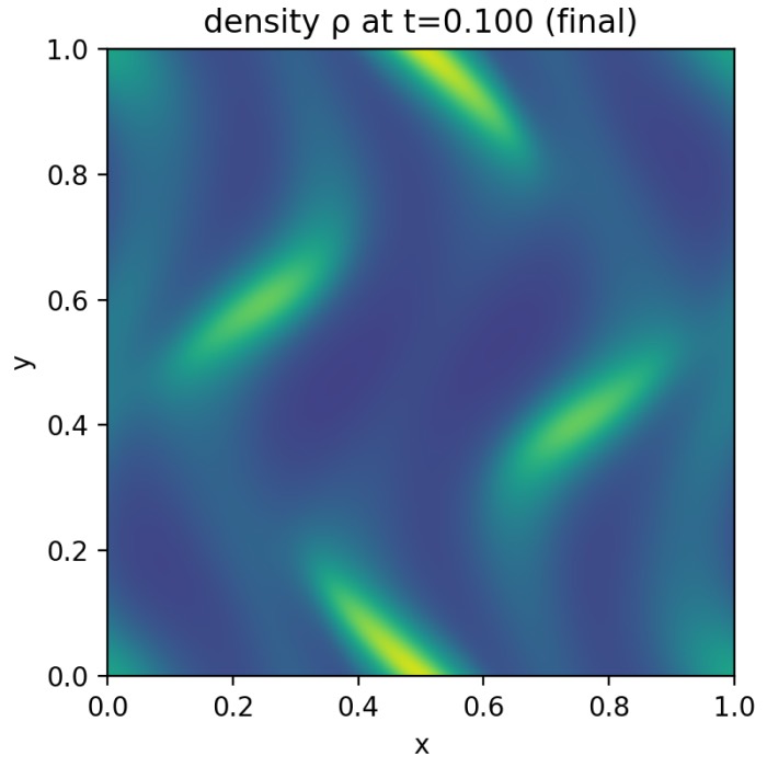
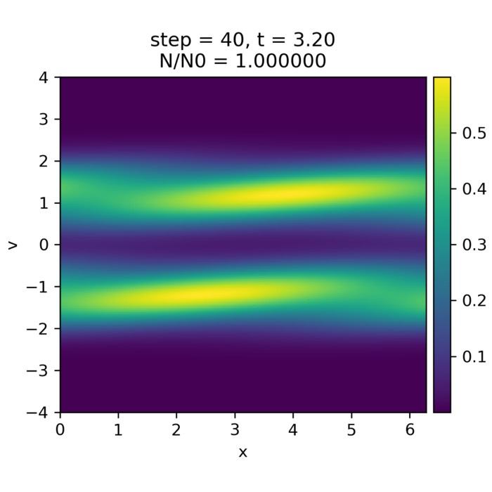
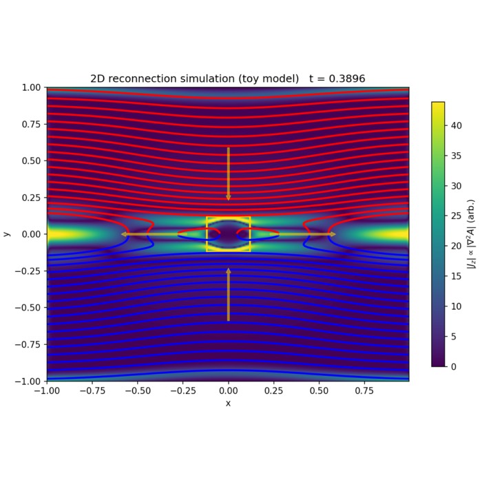
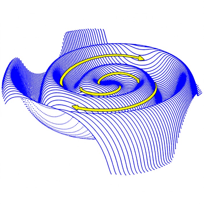
Final result of the MHD simulation from the numerical experiment we present in this post.
In this post, we summarize the standard MHD equations, explain what is meant by ideal MHD and Hall MHD, and discuss several key qualitative properties that are specific to MHD. At the end, we present a compact numerical experiment in Python that illustrates how complex structure can arise from the intrinsic nonlinearity of the MHD equations, even in a simple periodic box.
General MHD equations for an electrically conducting fluid
A common starting point is the fluid description coupled to Maxwell’s equations under the assumptions appropriate for non relativistic plasma dynamics. The set of equations presented here is written in a form that highlights the main physical terms.
The continuity equation enforces conservation of mass:
\[\begin{align} \partial_t \rho + \nabla\cdot(\rho \mathbf{v}) = 0 \end{align}\]with
- $\rho$ the mass density, and
- $\mathbf{v}$ the bulk flow velocity.
A momentum equation of Navier Stokes type describes the evolution of the bulk flow. In the most general fluid form one may write:
\[\begin{align} \rho\left(\partial_t \mathbf{v} + \mathbf{v}\cdot\nabla \mathbf{v}\right) = -\nabla\cdot\underline{\mathbf{P}} + \mathbf{j}\times\mathbf{B} + \mathbf{R} \end{align}\]Here,
- $\underline{\mathbf{P}}$ is the pressure tensor,
- $\mathbf{j}$ is the current density,
- $\mathbf{j}\times\mathbf{B}$ is the Lorentz force density, and
- $\mathbf{R}$ represents collisional friction terms or momentum exchange between species.
The induction equation follows from Faraday’s law together with a generalized Ohm’s law:
\[\begin{align} \partial_t \mathbf{B} = \nabla\times\left(\mathbf{v}\times\mathbf{B} - \eta \mathbf{j} + \frac{1}{en}(\mathbf{j}\times\mathbf{B})\right) \end{align}\]with
- $\mathbf{B}$ the magnetic field,
- $\eta$ the resistivity,
- $e$ the elementary charge, and
- $n$ the number density of charge carriers.
The term $-\eta\mathbf{j}$ corresponds to resistive diffusion, while $\frac{1}{en}(\mathbf{j}\times\mathbf{B})$ is the Hall term. The Hall term becomes relevant when ion and electron dynamics decouple on scales comparable to the ion inertial length. In many large scale heliospheric settings the Hall term is negligible, but in thin current sheets and reconnection layers it can be decisive.
To close the system one adds an equation of state. A frequently used choice is an adiabatic or polytropic relation:
\[\begin{align} p = p_0\left(\frac{\rho}{\rho_0}\right)^\gamma \end{align}\]where $p$ is the scalar pressure, $p_0$ and $\rho_0$ are reference pressure and density values, and $\gamma$ is the adiabatic index.
In addition, MHD assumes magnetic flux conservation in the sense that magnetic monopoles do not exist:
\[\begin{align} \nabla\cdot\mathbf{B} = 0 \end{align}\]The terms $\eta$, $\mathbf{R}$, and the Hall contribution define how far the plasma deviates from the idealized limit. When the conductivity is high, the resistivity is very small, and the plasma behaves approximately as an ideal conductor.
Ideal MHD
Ideal MHD is obtained by neglecting resistivity, collisional friction, and the Hall term:
\[\begin{align}\eta = 0,\; \mathbf{R}=0,\; \text{Hall term}=0 \end{align}\]The resulting system is:
Continuity:
\[\begin{align} \partial_t \rho + \nabla\cdot(\rho \mathbf{v}) = 0 \end{align}\]Momentum:
\[\begin{align} \rho\left(\partial_t \mathbf{v} + \mathbf{v}\cdot\nabla \mathbf{v}\right) = -\nabla\cdot\underline{\mathbf{P}} + \mathbf{j}\times\mathbf{B} \end{align}\]Induction:
\[\begin{align} \partial_t \mathbf{B} = \nabla\times(\mathbf{v}\times\mathbf{B}) \end{align}\]Equation of state:
\[\begin{align} p = p_0\left(\frac{\rho}{\rho_0}\right)^\gamma \end{align}\]The adjective ideal does not mean optimal. It means idealized. The approximation is appropriate when magnetic diffusion is negligible on the timescales of interest and when the plasma remains well described by a single fluid model.
Hall MHD
Hall MHD retains the Hall term in the induction equation while still neglecting resistivity and other non ideal effects:
Continuity:
\[\begin{align} \partial_t \rho + \nabla\cdot(\rho \mathbf{v}) = 0 \end{align}\]Momentum:
\[\begin{align} \rho\left(\partial_t \mathbf{v} + \mathbf{v}\cdot\nabla \mathbf{v}\right) = -\nabla\cdot\underline{\mathbf{P}} + \mathbf{j}\times\mathbf{B} \end{align}\]Induction with Hall term:
\[\begin{align} \partial_t \mathbf{B} = \nabla\times\left(\mathbf{v}\times\mathbf{B} + \frac{1}{en}(\mathbf{j}\times\mathbf{B})\right) \end{align}\]Equation of state:
\[\begin{align} p = p_0\left(\frac{\rho}{\rho_0}\right)^\gamma \end{align}\]Hall MHD modifies wave propagation and the small scale structure of current sheets. It is often used as an intermediate model between ideal MHD and fully kinetic plasma descriptions.
Key properties of MHD
The terms that are unique to MHD lead to a small number of qualitative principles that reappear throughout plasma physics. The items below are not additional assumptions. They are implications of the MHD equations under the relevant limits.
Magnetic pressure and magnetic tension
The Lorentz force density $\mathbf{j}\times\mathbf{B}$ is the essential coupling between field and flow. Using Ampère’s law in the MHD approximation, where the displacement current is neglected,
\[\begin{align} \nabla\times\mathbf{B} = \mu_0 \mathbf{j}, \end{align}\]one may rewrite the Lorentz force as a magnetic stress. A standard vector identity yields:
\[\begin{equation} \begin{aligned} \mathbf{j}\times\mathbf{B} &= \frac{1}{\mu_0}(\nabla\times\mathbf{B})\times\mathbf{B} \\ &= -\nabla\left(\frac{B^2}{2\mu_0}\right) + \frac{1}{\mu_0}(\mathbf{B}\cdot\nabla)\mathbf{B} \end{aligned} \end{equation}\]where $B^2 = \mathbf{B}\cdot\mathbf{B}$.
The decomposition highlights two physically distinct effects:
- Magnetic pressure: $p_B = \frac{B^2}{2\mu_0}$
- Magnetic tension: $\mathbf{t}_B = \frac{1}{\mu_0}(\mathbf{B}\cdot\nabla)\mathbf{B}$
Magnetic pressure acts like an isotropic pressure associated with field strength. Regions of enhanced magnetic field exert an effective pressure that drives plasma away from the strong field region. Magnetic tension acts like an elastic restoring force along field lines. It becomes important when field lines are curved. Curvature implies that the field line is under tension and tends to straighten, accelerating the plasma and transferring energy between flow and field.
This decomposition also clarifies why MHD can behave very differently from ordinary hydrodynamics. The fluid is not only accelerated by gradients of thermal pressure. It is also accelerated by gradients and curvature of the magnetic field.
Frozen in field theorem
The induction equation of ideal MHD,
\[\begin{align} \partial_t \mathbf{B} = \nabla\times(\mathbf{v}\times\mathbf{B}), \end{align}\]is equivalent to Faraday’s law $\partial_t \mathbf{B} = -\nabla\times\mathbf{E}$ together with the ideal Ohm’s law:
\[\begin{align} \mathbf{E} = -\mathbf{v}\times\mathbf{B} \end{align}\]In the limit of infinite conductivity, electric fields are shorted out in the rest frame of the plasma. For non relativistic velocities a Galilean transformation implies:
\[\begin{align} \mathbf{E}' = \mathbf{E} + \mathbf{v}\times\mathbf{B} \end{align}\]Thus, in the comoving frame of the plasma, ideal MHD implies $\mathbf{E}’ = 0$ and therefore again:
\[\begin{align} \mathbf{E} = -\mathbf{v}\times\mathbf{B} \end{align}\]A standard consequence is the frozen in field theorem: magnetic field lines move with the plasma. More precisely, the magnetic flux through any material surface comoving with the plasma is conserved. Let
\[\begin{align} \Phi = \iint_A \mathbf{B}\cdot d\mathbf{A} \end{align}\]denote the flux through a surface $A(t)$ that is transported by the flow. Under ideal MHD one can show:
\[\begin{align} \frac{d\Phi}{dt} = 0 \end{align}\]A useful differential statement of this idea is obtained by expanding the induction equation and combining it with the continuity equation. One finds:
\[\begin{align} d_t\left(\frac{\mathbf{B}}{\rho}\right) = \left(\frac{\mathbf{B}}{\rho}\cdot\nabla\right)\mathbf{v} \end{align}\]where $d_t = \partial_t + \mathbf{v}\cdot\nabla$ is the material derivative. This expression makes explicit that the magnetic field per unit mass behaves like a line element that is stretched and rotated by the velocity gradient tensor. In qualitative terms, plasma motion stretches and folds the magnetic field. Conversely, magnetic stresses feed back on the flow through the Lorentz force.
The frozen in statement has sharp limits. It requires ideal MHD conditions, which in practice means that resistive and other non ideal terms remain negligible on the scales and times of interest.
No electric fields parallel to the magnetic field in ideal MHD
From the ideal Ohm’s law,
\[\begin{align} \mathbf{E} = -\mathbf{v}\times\mathbf{B}, \end{align}\]it follows immediately that
\[\begin{align} \mathbf{E}\cdot\mathbf{B} = 0 \end{align}\]and therefore the component of the electric field parallel to the magnetic field vanishes:
\[\begin{align} \mathbf{E}_\parallel = 0 \end{align}\]This matters because parallel electric fields are required for direct acceleration of charged particles along field lines. Phenomena such as auroral particle acceleration therefore require physics beyond ideal MHD, for example finite conductivity, electron inertia, or kinetic effects.
No electric field in the plasma rest frame
As already used in the frozen in argument, ideal MHD implies that in the comoving frame:
\[\begin{align} \mathbf{E}' = 0 \end{align}\]This is a rest frame statement. In the laboratory frame $\mathbf{E}$ can be nonzero, but it is fully determined by the bulk motion through $-\mathbf{v}\times\mathbf{B}$.
Topology conservation of magnetic field lines
In ideal MHD, the frozen in theorem implies a strong topological constraint. Since field lines are transported with the flow and flux through material surfaces is conserved, the connectivity of field lines is preserved. In practical terms:
- Closed magnetic field lines remain closed.
- Field line connectivity does not change.
This is not merely a geometric statement. It is a statement about the inability of ideal MHD to change magnetic topology. Reconnection, in which field lines break and reconnect, necessarily requires non ideal effects. In numerical simulations of ideal MHD one may still see strong current sheets that look like reconnection layers, but true topological change is formally excluded by the model and would occur only through numerical diffusion.
Magnetic Reynolds number
To quantify when ideal MHD is justified, it is useful to compare inductive advection with resistive diffusion. Using $\mathbf{j} = \frac{1}{\mu_0}\nabla\times\mathbf{B}$ and assuming constant conductivity $\sigma$ with $\eta = \frac{1}{\mu_0\sigma}$, the induction equation with resistivity can be written schematically as:
\[\begin{align} \partial_t \mathbf{B} \approx \nabla\times(\mathbf{v}\times\mathbf{B}) + \eta \nabla^2 \mathbf{B} \end{align}\]A scale analysis with characteristic length $L$, speed $v$, and timescale $\tau$ gives:
\[\begin{align} \frac{B}{\tau} \sim \frac{vB}{L} + \eta\frac{B}{L^2} \end{align}\]The ratio of the advective term to the diffusive term defines the magnetic Reynolds number:
\[\begin{align} R_M = \frac{vL}{\eta} = \mu_0\sigma Lv \end{align}\]The interpretation is:
- If $R_M \gg 1$, diffusion is negligible, flux freezing holds approximately, and ideal MHD is a good approximation.
- If $R_M \sim 1$, diffusion competes with advection, the frozen in picture breaks down, and magnetic topology can change.
In many space plasma environments, $R_M$ is extremely large on macroscopic scales. This is the origin of the pervasive usefulness of ideal MHD for large scale structure. At the same time, reconnection and dissipation occur in localized thin layers where effective diffusivities and small scales can reduce the relevant magnetic Reynolds number.
Numerical example in Python
To illustrate the qualitative dynamics of magnetohydrodynamic plasmas, we consider a simple two-dimensional numerical experiment based on the equations of ideal MHD. The simulation is not intended as a high-fidelity space plasma model, but as a compact and transparent demonstration of how nonlinear plasma and magnetic field dynamics arise even in strongly simplified settings.
Physical model
The plasma is described within the framework of ideal MHD, treating it as a single, electrically conducting fluid characterized by mass density $\rho$, bulk velocity $\mathbf{v}$, thermal pressure $p$, and magnetic field $\mathbf{B}$. Dissipative effects such as viscosity, resistivity, radiation losses, or kinetic physics are neglected. As a consequence, the model captures only large-scale, fluid-like plasma behavior and magnetic field evolution.
The governing equations are solved in conservative form for the variables
\[U = \left(\rho,; \rho v_x,; \rho v_y,; \rho v_z,; E,; B_x,; B_y,; B_z,; \psi\right),\]where $E$ is the total energy density and $\psi$ is an auxiliary scalar field introduced for divergence control of the magnetic field.
The adiabatic index is fixed to $\gamma = 5/3$, corresponding to a monoatomic ideal gas, as commonly assumed in space and astrophysical plasma contexts.
Dimensionality, geometry, and boundary conditions
The simulation is carried out in two spatial dimensions on a uniform Cartesian grid covering a square domain $[0,1]\times[0,1]$. All fields depend on $(x,y)$ only, while vector quantities may still have out-of-plane components. The magnetic field is initialized entirely in-plane, so that the out-of-plane current density
\[j_z = (\nabla \times \mathbf{B})_z\]serves as a useful diagnostic for the formation of current sheets.
Periodic boundary conditions are applied in both spatial directions. There are no solid boundaries, obstacles, internal conductors, or material interfaces. The domain represents an unbounded, homogeneous plasma volume tiled periodically in space. Consequently, all observed structures arise self-consistently from the intrinsic nonlinear dynamics of the MHD equations rather than from interactions with external objects or imposed geometries.
Initial condition: Orszag–Tang vortex
As an initial condition, we employ the classical Orszag–Tang vortex, a standard benchmark problem in MHD. It consists of smooth, large-scale sinusoidal velocity and magnetic field patterns that are not mutually aligned. Specifically, the velocity and magnetic field are initialized as
\[\begin{align*} \mathbf{v}(x,y) &= \big(-\sin(2\pi y), \sin(2\pi x), 0\big), \\ \mathbf{B}(x,y) &= \big(-\sin(2\pi y), \sin(4\pi x), 0\big), \end{align*}\]with uniform density and pressure.
Although the initial state is smooth and free of discontinuities, it is dynamically unstable under MHD evolution. The misalignment between flow and magnetic field leads to rapid nonlinear coupling, magnetic field line stretching, compression, and the spontaneous formation of sharp gradients. This makes the Orszag–Tang vortex particularly suitable for demonstrating how complex plasma structures emerge from simple initial conditions.
Numerical method
The MHD equations are discretized using a finite-volume formulation with a Rusanov (local Lax–Friedrichs) flux. This choice prioritizes robustness and simplicity over low numerical diffusion. Time integration is performed using a second-order Runge–Kutta scheme (RK2), with the time step dynamically adjusted according to a Courant–Friedrichs–Lewy (CFL) condition based on the fast magnetosonic wave speed.
To control numerical violations of the solenoidal constraint $\nabla\cdot\mathbf{B}=0$, a Generalized Lagrange Multiplier (GLM) divergence cleaning scheme is employed. The auxiliary field $\psi$ propagates divergence errors away from their point of origin while simultaneously damping them on a prescribed timescale. This approach avoids the complexity of constrained transport while keeping $\nabla\cdot\mathbf{B}$ sufficiently small for the purposes of this demonstration.
Diagnostics and visualization
During the simulation, snapshots of the plasma state are recorded at regular intervals. We visualize:
- the mass density $\rho(x,y)$, highlighting compressive and rarefactive structures produced by the coupled plasma–field dynamics,
- the out-of-plane current density proxy $j_z = \partial_x B_y - \partial_y B_x$, which reveals the formation of thin current sheets associated with strong magnetic field gradients.
Both quantities are plotted using fixed color scales to allow direct visual comparison across time. In addition to saving individual frames, the simulation produces an animated sequence that illustrates the continuous evolution from smooth initial conditions to a strongly structured MHD state.
Scope and limitations
It is important to emphasize what this numerical example does and does not represent. The simulation does not model a specific astrophysical or planetary plasma environment, nor does it include obstacles, ionospheres, bow shocks, or magnetospheres. Effects such as reconnection physics, particle acceleration, or kinetic scales are not resolved. The example instead serves as a controlled illustration of how ideal MHD alone already produces current sheets, density contrasts, and complex spatiotemporal structure.
In this sense, the simulation should be read as a conceptual demonstration of MHD dynamics rather than as a predictive physical model. Its value lies in making the abstract coupling between fluid motion and magnetic fields directly visible in a minimal, reproducible Python implementation.
Python implementation
We begin by importing the necessary libraries:
import numpy as np
import matplotlib.pyplot as plt
import os
import imageio.v2 as imageio
from PIL import Image
import glob
Next, we define functions to convert between primitive and conservative variables, compute fluxes, and calculate the fast magnetosonic speed:
def prim_to_cons(rho, vx, vy, vz, p, Bx, By, Bz, psi, gamma):
    kinetic = 0.5 * rho * (vx*vx + vy*vy + vz*vz)
    mag = 0.5 * (Bx*Bx + By*By + Bz*Bz)
    E = p/(gamma - 1.0) + kinetic + mag + 0.5 * psi*psi
    mx = rho * vx
    my = rho * vy
    mz = rho * vz
    return np.stack([rho, mx, my, mz, E, Bx, By, Bz, psi], axis=0)

def cons_to_prim(U, gamma):
    rho = U[0]
    mx, my, mz = U[1], U[2], U[3]
    E = U[4]
    Bx, By, Bz = U[5], U[6], U[7]
    psi = U[8]

    vx = mx / rho
    vy = my / rho
    vz = mz / rho

    kinetic = 0.5 * rho * (vx*vx + vy*vy + vz*vz)
    mag = 0.5 * (Bx*Bx + By*By + Bz*Bz)
    p = (gamma - 1.0) * (E - kinetic - mag - 0.5*psi*psi)

    return rho, vx, vy, vz, p, Bx, By, Bz, psi

def flux_x(U, gamma):
    rho, vx, vy, vz, p, Bx, By, Bz, psi = cons_to_prim(U, gamma)
    mx, my, mz = U[1], U[2], U[3]
    E = U[4]

    B2 = Bx*Bx + By*By + Bz*Bz
    vB = vx*Bx + vy*By + vz*Bz
    pt = p + 0.5*B2

    # GLM coupling
    # In x-direction: Bx flux gets psi, psi flux gets c_h^2 * Bx
    # c_h is handled outside in Rusanov signal speed and psi flux below
    Fx = np.empty_like(U)
    Fx[0] = mx
    Fx[1] = mx*vx + pt - Bx*Bx
    Fx[2] = my*vx - Bx*By
    Fx[3] = mz*vx - Bx*Bz
    Fx[4] = (E + pt)*vx - Bx*vB
    Fx[5] = 0.0      # replaced later by +psi in Rusanov interface form
    Fx[6] = By*vx - Bx*vy
    Fx[7] = Bz*vx - Bx*vz
    Fx[8] = 0.0      # replaced later by c_h^2 * Bx
    return Fx

def flux_y(U, gamma):
    rho, vx, vy, vz, p, Bx, By, Bz, psi = cons_to_prim(U, gamma)
    mx, my, mz = U[1], U[2], U[3]
    E = U[4]

    B2 = Bx*Bx + By*By + Bz*Bz
    vB = vx*Bx + vy*By + vz*Bz
    pt = p + 0.5*B2

    Fy = np.empty_like(U)
    Fy[0] = my
    Fy[1] = mx*vy - By*Bx
    Fy[2] = my*vy + pt - By*By
    Fy[3] = mz*vy - By*Bz
    Fy[4] = (E + pt)*vy - By*vB
    Fy[5] = Bx*vy - By*vx
    Fy[6] = 0.0      # replaced later by +psi in Rusanov interface form
    Fy[7] = Bz*vy - By*vz
    Fy[8] = 0.0      # replaced later by c_h^2 * By
    return Fy

def fast_magnetosonic_speed(rho, p, Bx, By, Bz, gamma, nx, ny):
    # Directional fast speed approximation.
    # c_f^2 = 0.5 * (a^2 + vA^2 + sqrt((a^2 + vA^2)^2 - 4 a^2 vAn^2))
    a2 = gamma * p / rho
    B2 = Bx*Bx + By*By + Bz*Bz
    vA2 = B2 / rho
    Bn = Bx*nx + By*ny
    vAn2 = (Bn*Bn) / rho
    term = (a2 + vA2)**2 - 4.0*a2*vAn2
    term = np.maximum(term, 0.0)
    cf2 = 0.5 * (a2 + vA2 + np.sqrt(term))
    return np.sqrt(np.maximum(cf2, 0.0))

def rusanov_flux_x(UL, UR, gamma, c_h):
    FL = flux_x(UL, gamma)
    FR = flux_x(UR, gamma)

    # Insert GLM components in x-direction
    # Bx flux = psi, psi flux = c_h^2 * Bx
    FL = FL.copy()
    FR = FR.copy()
    FL[5] = UL[8]
    FR[5] = UR[8]
    FL[8] = (c_h*c_h) * UL[5]
    FR[8] = (c_h*c_h) * UR[5]

    # Signal speed
    rL, vLx, vLy, vLz, pL, BLx, BLy, BLz, psiL = cons_to_prim(UL, gamma)
    rR, vRx, vRy, vRz, pR, BRx, BRy, BRz, psiR = cons_to_prim(UR, gamma)

    cfL = fast_magnetosonic_speed(rL, pL, BLx, BLy, BLz, gamma, 1.0, 0.0)
    cfR = fast_magnetosonic_speed(rR, pR, BRx, BRy, BRz, gamma, 1.0, 0.0)
    smax = np.maximum(np.abs(vLx) + cfL, np.abs(vRx) + cfR)
    smax = np.maximum(smax, c_h)

    return 0.5*(FL + FR) - 0.5*smax*(UR - UL)

def rusanov_flux_y(UL, UR, gamma, c_h):
    FL = flux_y(UL, gamma)
    FR = flux_y(UR, gamma)

    # Insert GLM components in y-direction
    # By flux = psi, psi flux = c_h^2 * By
    FL = FL.copy()
    FR = FR.copy()
    FL[6] = UL[8]
    FR[6] = UR[8]
    FL[8] = (c_h*c_h) * UL[6]
    FR[8] = (c_h*c_h) * UR[6]

    rL, vLx, vLy, vLz, pL, BLx, BLy, BLz, psiL = cons_to_prim(UL, gamma)
    rR, vRx, vRy, vRz, pR, BRx, BRy, BRz, psiR = cons_to_prim(UR, gamma)

    cfL = fast_magnetosonic_speed(rL, pL, BLx, BLy, BLz, gamma, 0.0, 1.0)
    cfR = fast_magnetosonic_speed(rR, pR, BRx, BRy, BRz, gamma, 0.0, 1.0)
    smax = np.maximum(np.abs(vLy) + cfL, np.abs(vRy) + cfR)
    smax = np.maximum(smax, c_h)

    return 0.5*(FL + FR) - 0.5*smax*(UR - UL)
We then define functions for periodic padding,
def periodic_pad(U):
    # U: (nvars, ny, nx)
    return np.pad(U, ((0,0),(1,1),(1,1)), mode="wrap")
computing the right-hand side of the MHD equations,
def compute_rhs(U, dx, dy, gamma, c_h, c_p):
    # GLM damping: psi_t += - (c_h^2 / c_p^2) psi
    # We'll apply as a source term.
    Up = periodic_pad(U)
    nvars, ny, nx = U.shape

    # Fluxes at interfaces
    Fx = np.zeros((nvars, ny, nx+1), dtype=U.dtype)
    Fy = np.zeros((nvars, ny+1, nx), dtype=U.dtype)

    # x-interfaces
    for i in range(nx+1):
        UL = Up[:, 1:-1, i]     # left cell at interface
        UR = Up[:, 1:-1, i+1]   # right cell
        Fx[:, :, i] = rusanov_flux_x(UL, UR, gamma, c_h)

    # y-interfaces
    for j in range(ny+1):
        UL = Up[:, j, 1:-1]
        UR = Up[:, j+1, 1:-1]
        Fy[:, j, :] = rusanov_flux_y(UL, UR, gamma, c_h)

    rhs = np.zeros_like(U)
    rhs -= (Fx[:, :, 1:] - Fx[:, :, :-1]) / dx
    rhs -= (Fy[:, 1:, :] - Fy[:, :-1, :]) / dy

    # psi damping source
    rhs[8] += -(c_h*c_h / (c_p*c_p)) * U[8]
    return rhs
and performing a single RK2 time step:
def step_rk2(U, dt, dx, dy, gamma, c_h, c_p):
    k1 = compute_rhs(U, dx, dy, gamma, c_h, c_p)
    U1 = U + dt*k1
    k2 = compute_rhs(U1, dx, dy, gamma, c_h, c_p)
    return 0.5*(U + U1 + dt*k2)
Then, we set up the initial condition for the Orszag–Tang vortex:
def orszag_tang_ic(nx, ny, gamma):
    # Domain [0, 1] x [0, 1]
    x = (np.arange(nx) + 0.5) / nx
    y = (np.arange(ny) + 0.5) / ny
    X, Y = np.meshgrid(x, y, indexing="xy")

    rho = np.ones((ny, nx))
    p = (gamma - 1.0) * np.ones((ny, nx))  # common choice

    vx = -np.sin(2.0*np.pi*Y)
    vy =  np.sin(2.0*np.pi*X)
    vz = np.zeros_like(vx)

    Bx = -np.sin(2.0*np.pi*Y)
    By =  np.sin(4.0*np.pi*X)
    Bz = np.zeros_like(Bx)

    psi = np.zeros_like(rho)
    U = prim_to_cons(rho, vx, vy, vz, p, Bx, By, Bz, psi, gamma)
    return U
We also define a function to compute the time step based on the CFL condition:
def compute_dt(U, dx, dy, gamma, cfl, c_h):
    rho, vx, vy, vz, p, Bx, By, Bz, psi = cons_to_prim(U, gamma)
    cf_x = fast_magnetosonic_speed(rho, p, Bx, By, Bz, gamma, 1.0, 0.0)
    cf_y = fast_magnetosonic_speed(rho, p, Bx, By, Bz, gamma, 0.0, 1.0)
    smax_x = np.max(np.abs(vx) + cf_x)
    smax_y = np.max(np.abs(vy) + cf_y)
    smax_x = max(smax_x, c_h)
    smax_y = max(smax_y, c_h)
    dt = cfl / (smax_x/dx + smax_y/dy + 1e-14)
    return dt
Finally, we set the simulation parameters and run the time-stepping loop, saving frames for visualization:
gamma = 5.0/3.0

# set grid size and resolution:
nx, ny = 256, 256
dx, dy = 1.0/nx, 1.0/ny

# GLM parameters:
c_h = 1.0
c_p = 0.2

cfl = 0.4
t_end = 0.5 # increase for more dynamic evolution (but longer runtime)

# output settings:
out_dir = "frames"
os.makedirs(out_dir, exist_ok=True)

plot_every = 20
dpi = 200

gif_path = os.path.join(out_dir, "mhd_evolution.gif")
gif_fps = 10   # frames per second in GIF

frame_files = []   # collect frame paths here

U = orszag_tang_ic(nx, ny, gamma)

t = 0.0
it = 0

# prepare GIF writer:
gif_path = os.path.join(out_dir, "mhd_evolution.gif")
gif_fps = 10
gif_writer = imageio.get_writer(gif_path, mode="I", fps=gif_fps)

# main time-stepping loop
while t < t_end:
    dt = compute_dt(U, dx, dy, gamma, cfl, c_h)
    if t + dt > t_end:
        dt = t_end - t

    U = step_rk2(U, dt, dx, dy, gamma, c_h, c_p)
    t += dt
    it += 1

    if it % plot_every == 0 or t >= t_end:
        rho, vx, vy, vz, p, Bx, By, Bz, psi = cons_to_prim(U, gamma)

        divB_rms = np.sqrt(np.mean(
            ((np.roll(Bx, -1, axis=1) - np.roll(Bx, 1, axis=1))/(2*dx) +
             (np.roll(By, -1, axis=0) - np.roll(By, 1, axis=0))/(2*dy))**2))

        print(f"t={t:.4f}, dt={dt:.3e}, iter={it}, divB_rms~{divB_rms:.3e}")

        dBy_dx = (np.roll(By, -1, axis=1) - np.roll(By, 1, axis=1)) / (2*dx)
        dBx_dy = (np.roll(Bx, -1, axis=0) - np.roll(Bx, 1, axis=0)) / (2*dy)
        jz = dBy_dx - dBx_dy

        fig, ax = plt.subplots(1, 2, figsize=(10, 4), constrained_layout=True)

        im0 = ax[0].imshow(rho, origin="lower", extent=(0, 1, 0, 1), vmin=0, vmax=3)
        ax[0].set_title(f"density ρ at t={t:.3f} (iter {it})")
        ax[0].set_xlabel("x")
        ax[0].set_ylabel("y")
        plt.colorbar(im0, ax=ax[0], fraction=0.046, pad=0.04)

        im1 = ax[1].imshow(jz, origin="lower", extent=(0, 1, 0, 1), vmin=-60, vmax=70)
        ax[1].set_title("current proxy jz = ∂x By − ∂y Bx")
        ax[1].set_xlabel("x")
        ax[1].set_ylabel("y")
        plt.colorbar(im1, ax=ax[1], fraction=0.046, pad=0.04)

        frame_path = os.path.join(out_dir, f"frame_{len(frame_files):06d}.png")
        plt.savefig(frame_path, dpi=dpi)

        # append to GIF:
        fig.canvas.draw()
        w, h = fig.canvas.get_width_height()
        buf = np.frombuffer(fig.canvas.buffer_rgba(), dtype=np.uint8).reshape(h, w, 4)
        rgb = buf[:, :, :3]  # Convert RGBA to RGB
        gif_writer.append_data(rgb)

        plt.close(fig)

        frame_files.append(frame_path)

# finalize the GIF:
print("Creating GIF...")
gif_writer.close()
print(f"GIF written to {gif_path}")
Discussion of the simulation results
The resulting GIF shows the time evolution of a two dimensional ideal MHD simulation initialized with the Orszag Tang vortex. Left panel: mass density $\rho(x,y,t)$, visualizing compressions and rarefactions produced by the nonlinear coupling between flow and magnetic stresses. Right panel: out of plane current density proxy $j_z(x,y,t) = \partial_x B_y - \partial_y B_x$, highlighting thin current sheets where magnetic field gradients become large. The domain is a periodic square $[0,1]\times[0,1]$ with no obstacles or boundaries. The numerical scheme is a finite volume method with a Rusanov flux and RK2 time stepping; $\nabla\cdot\mathbf{B}$ is controlled by GLM divergence cleaning via the auxiliary field $\psi$. Color scales are held fixed across frames to make structural growth comparable over time.
The animated evolution is a compact demonstration of what makes MHD qualitatively different from ordinary hydrodynamics. Even though the initial condition is smooth and contains only large scale sinusoidal modes, the coupled MHD dynamics rapidly generates sharp gradients, filamentary structures, and strong spatial intermittency. None of these patterns are imposed by boundaries or obstacles. They arise solely from the internal feedback between the induction equation, which transports and deforms $\mathbf{B}$ with the flow, and the momentum equation, which responds to magnetic pressure and magnetic tension forces.
A useful way to read the left panel is to treat $\rho(x,y,t)$ as a tracer of compressibility and shock like structures. In the Orszag Tang setup, the initial velocity field and magnetic field are deliberately misaligned. This causes the flow to stretch and fold the magnetic field while simultaneously being accelerated by magnetic stresses. The result is the formation of compressive regions where the density increases and evacuated regions where it decreases. In ideal MHD the only mechanism that produces such density contrasts is the nonlinear interplay of advective compression, pressure response through the chosen equation of state, and magnetosonic wave dynamics. The emergence of sharp density features therefore indicates that the system has moved far into the nonlinear regime, where wave steepening and shock formation become important even without explicit viscosity.
The right panel, showing $j_z = \partial_x B_y - \partial_y B_x$, is even more diagnostic of the characteristic MHD behavior. Because $j_z$ is the curl of the in plane magnetic field, large magnitude values correspond to regions where $\mathbf{B}$ varies rapidly in space. The animation reveals the spontaneous appearance of thin, intense current filaments and sheets. This is the typical route by which smooth magnetic fields evolve under ideal like dynamics: advection and stretching concentrate gradients until they are limited by dissipation. In a strictly ideal model physical resistivity is absent, so true magnetic reconnection and true topological change are not part of the continuum equations. Nevertheless, the simulation exhibits the geometric precursors of reconnection, namely the formation of narrow current sheets that would become reconnection sites in more complete models that include resistivity, Hall physics, or kinetic effects. In practical numerical schemes, some effective reconnection can still occur through numerical diffusion, but the conceptual point remains: current sheet formation is an intrinsic outcome of the MHD nonlinearity.
The periodic boundary conditions matter for interpretation. Since the domain is periodic and contains no obstacles, there is no preferred location or externally imposed direction. Structures appear and interact throughout the domain. The animation therefore illustrates a homogeneous self organized evolution rather than a driven interaction region as in planetary magnetospheres or lunar wakes. For the purposes of our post, this is a feature. It isolates the internal mechanism by which MHD creates structure, without conflating it with boundary forcing, inflow conditions, or obstacle physics.
The diagnostic printed during the run, the root mean square of $\nabla\cdot\mathbf{B}$ estimated from finite differences, typically stays small compared to the characteristic gradients in $\mathbf{B}$:
...
t=0.4358, dt=3.135e-04, iter=1500, divB_rms~5.100e-02
t=0.4420, dt=3.149e-04, iter=1520, divB_rms~5.035e-02
t=0.4484, dt=3.165e-04, iter=1540, divB_rms~4.962e-02
t=0.4547, dt=3.183e-04, iter=1560, divB_rms~4.890e-02
t=0.4611, dt=3.202e-04, iter=1580, divB_rms~4.818e-02
t=0.4675, dt=3.221e-04, iter=1600, divB_rms~4.742e-02
t=0.4739, dt=3.217e-04, iter=1620, divB_rms~4.662e-02
t=0.4804, dt=3.212e-04, iter=1640, divB_rms~4.579e-02
t=0.4868, dt=3.207e-04, iter=1660, divB_rms~4.502e-02
t=0.4932, dt=3.203e-04, iter=1680, divB_rms~4.437e-02
t=0.4996, dt=3.194e-04, iter=1700, divB_rms~4.386e-02
t=0.5000, dt=7.725e-05, iter=1702, divB_rms~4.383e-02
Creating GIF...
GIF written to frames/mhd_evolution.gif
This reflects the role of GLM divergence cleaning in propagating and damping divergence errors. The method is not as strict as constrained transport, but it is adequate for a robust educational example. The main visible physics in the GIF is not driven by divergence errors but by the intended ideal MHD coupling.
Finally, it is worth being explicit about what you should and should not conclude from the animation. The simulation does demonstrate that ideal MHD already predicts the emergence of compressive structures and thin current sheets from smooth initial conditions. It does not, by itself, determine the microphysics of dissipation, particle heating, or reconnection rates. Those require either explicit non ideal terms or kinetic modeling. In that sense, our simulation is best read as an illustration of the macroscopic route by which magnetized fluids naturally generate localized regions where the ideal approximation becomes least trustworthy, which is precisely why MHD systems so often concentrate dissipation into thin, spatially intermittent structures.
For a more detailed exploration of MHD numerical methods, including higher order schemes, constrained transport, and resistive effects, please refer to dedicated computational MHD packages such as
- Gawainꜛ: A 2D/3D magnetohydrodynamic simulation code written in Python that support 2D/3D inviscid, compressible hydrodynamics and 2D/3D ideal magnetohydrodynamics
- AMUN Codeꜛ: A high-performance code for numerical simulations of astrophysical plasmas. I saw that it contains both Fortran core routines a Python interface.
- PLUTOꜛ: A versatile and widely used astrophysical fluid dynamics code that supports MHD simulations. It is written in C and Fortran, with Python interfaces available for pre- and post-processing.
- Athena++ꜛ: A grid-based code for astrophysical MHD simulations. It is written in C++ and supports a variety of physics modules.
- ZEUS-MPꜛ: An MHD code designed for astrophysical applications, written in Fortran.
Concluding remarks
MHD is best understood as a theory of coupled stresses and constraints. Magnetic pressure and tension provide additional forces beyond hydrodynamics, while the induction equation imposes a strong link between flow and field, summarized by the frozen in picture and its topological consequences. These principles are not decorative. They determine which processes are possible in the ideal limit and which require non ideal physics.
The Python toy simulation demonstrates a central practical lesson: even in a periodic box with smooth initial conditions and without any obstacles or boundary forcing, the nonlinear MHD coupling rapidly produces sharp gradients and filamentary current structures. In real plasmas, such structures are precisely where dissipation and reconnection concentrate. Ideal MHD cannot fully capture that microphysics, but it already explains why current sheets and strong inhomogeneities are natural outcomes of magnetized fluid dynamics.
Update and code availability: This post and its accompanying Python code were originally drafted in 2020 and archived during the migration of this website to Jekyll and Markdown. In January 2026, I substantially revised and extended the code. The updated and cleaned-up implementation is now available in this new GitHub repositoryꜛ. Please feel free to experiment with it and to share any feedback or suggestions for further improvements.


comments