Vlasov–Poisson dynamics: Landau damping and the two-stream instability

In our previous discussion of kinetic plasma theory, the Vlasov equation emerged as the fundamental description of collisionless plasmas. Unlike fluid or magnetohydrodynamic models, which evolve a small number of velocity moments, the kinetic approach follows the full phase-space distribution function $f(x,v,t)$. This enables the description of phenomena that are intrinsically velocity-space dependent and therefore inaccessible to fluid models.

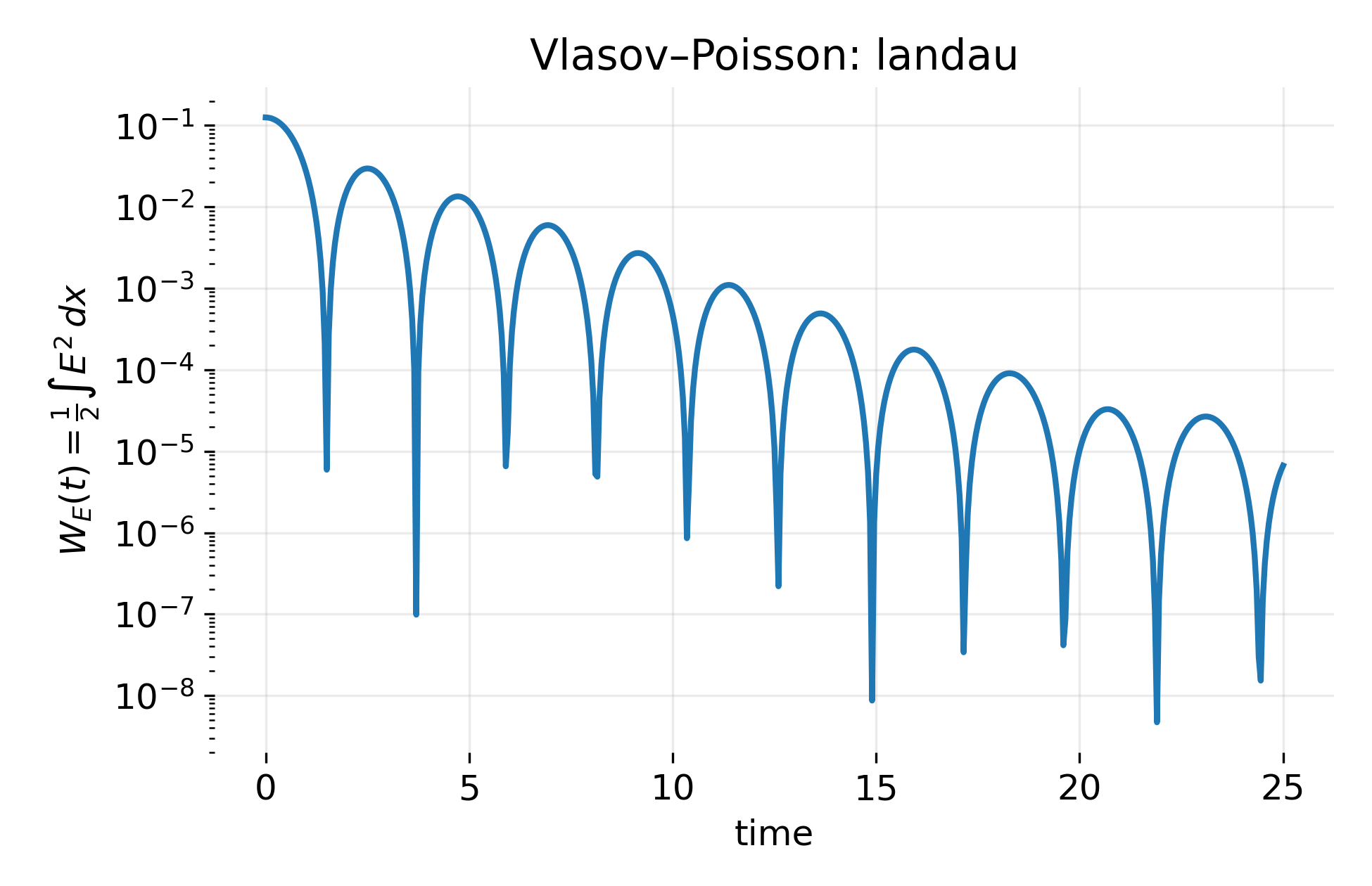
Energy evolution in the Vlasov–Poisson system for Landau damping. In this post, we explore how different initial velocity distributions lead to qualitatively distinct macroscopic dynamics, illustrating the inherently kinetic nature of these processes.

The numerical examples discussed ins this post illustrate this point. Using the one-dimensional Vlasov–Poisson system as a minimal setting, two canonical kinetic processes are demonstrated: Landau damping and the two-stream instability. Both arise from the same equations, differ only in the initial velocity distribution, and yet lead to qualitatively distinct macroscopic behavior.

The Vlasov–Poisson system as a minimal kinetic model

We consider an electrostatic, collisionless plasma in one spatial dimension $x$ and one velocity dimension $v$. The evolution of the electron distribution function is governed by the Vlasov equation

\[\partial_t f + v,\partial_x f + E(x,t),\partial_v f = 0 ,\]

where $E(x,t)$ is the self-consistent electric field. This equation expresses the conservation of phase-space density along particle trajectories,

\[\frac{Df}{Dt} = 0,\]

which is a direct manifestation of Liouville’s theorem for Hamiltonian dynamics.

The electric field is determined self-consistently from Poisson’s equation,

\[\partial_x E = 1 - n(x,t), \quad n(x,t) = \int f(x,v,t)\,dv,\]

where a uniform, immobile ion background of unit density ensures overall charge neutrality.

Despite its apparent simplicity, this system already captures the essential structure of kinetic plasma dynamics: nonlinear phase-space advection, wave–particle interaction, and energy exchange between particles and fields.

Phase-space advection and the meaning of collisionless dynamics

In the absence of collisions, the Vlasov equation describes pure advection in phase space. Phase-space elements may stretch, shear, and fold, but their volume is conserved. Apparent dissipation at the macroscopic level therefore does not correspond to entropy production or collisional relaxation, but to the redistribution of information into increasingly fine phase-space structure.

This geometric viewpoint is crucial for interpreting both Landau damping and kinetic instabilities. In both cases, the electric field exchanges energy with specific velocity classes of particles, while the total phase-space density remains conserved.

Landau damping: Damping without dissipation

The first application considers Landau damping, a phenomenon that is often counterintuitive from a fluid perspective. The system is initialized with a nearly Maxwellian velocity distribution and a small spatial density modulation,

\[f(x,v,0) = \left[ 1 + \alpha \cos(kx) \right] f_M(v),\]

where $\alpha \ll 1$ and $f_M(v)$ is a Maxwellian.

As the system evolves, an electrostatic plasma wave is excited. Linear theory predicts that the amplitude of this wave decays exponentially in time, even though the dynamics is strictly collisionless. This decay is not caused by friction or resistivity, but by resonant interaction between the wave and particles whose velocities are close to the phase velocity of the wave.

From a kinetic viewpoint, Landau damping corresponds to phase mixing in velocity space. Different velocity classes advect the initial perturbation at different rates, producing increasingly fine filamentation in $v$. While the electric field amplitude decreases, the perturbation energy is transferred into unresolved velocity-space structure rather than being dissipated.

This behavior is visible numerically in two complementary diagnostics. The electric field energy

\[W_E(t) = \frac{1}{2} \int E^2(x,t),dx\]

shows a damped oscillatory decay, while the perturbation distribution

\[\delta f(x,v,t) = f(x,v,t) - \langle f \rangle_x(v)\]

develops ever finer velocity-space filaments. The latter makes explicit that damping is accompanied by increasing phase-space complexity, not by relaxation toward a smoother state.

The two-stream instability: Extracting free energy from velocity space

The second application uses the same Vlasov–Poisson equations, but a qualitatively different initial condition. Instead of a single Maxwellian, the velocity distribution is bimodal,

\[f(x,v,0) = \left[ 1 + \alpha \cos(kx) \right] \frac{1}{2}\bigl[f_M(v-u) + f_M(v+u)\bigr],\]

representing two counter-streaming particle populations.

This distribution contains free energy stored in velocity space. Small electrostatic perturbations can tap into this energy, leading to exponential growth of the electric field. This is the classical two-stream instability.

In contrast to Landau damping, the electric field energy grows rather than decays, until nonlinear effects set in. As the instability develops, particles become trapped in the self-generated electrostatic potential wells. This trapping redistributes particles in velocity space, flattening the distribution near the resonant velocities and ultimately saturating the instability.

Phase-space snapshots reveal the characteristic deformation of the two beams: initially distinct streams are bent, broadened, and partially merged through nonlinear wave–particle interaction. The perturbation distribution $\delta f$ exhibits coherent, growing structures rather than fine filamentation, reflecting the fundamentally different nature of the dynamics.

Why these examples are inherently kinetic

Both Landau damping and the two-stream instability arise from the same collisionless equations and differ only in their initial velocity distributions. Their radically different macroscopic behavior illustrates why kinetic theory is indispensable for plasma physics.

Neither effect can be captured by fluid or MHD models, which eliminate velocity-space structure by construction. Landau damping requires a continuous velocity distribution and resonant wave–particle interaction, while the two-stream instability depends explicitly on non-thermal features of $f(v)$. In both cases, the decisive physics resides in phase space rather than configuration space.

The Vlasov–Poisson system thus provides a minimal yet powerful framework for demonstrating how microscopic phase-space dynamics gives rise to macroscopic plasma behavior.

Numerical implementation

The following Python code implements a semi-Lagrangian scheme to solve the 1D1V Vlasov–Poisson system described above (one-dimensional, collisionless plasma in phase space $(x,v)$). The code initializes either a Landau damping or two-stream instability scenario (same numerical core is used for both examples), evolves the distribution function using Strang splitting, and computes diagnostics such as electric field energy and phase-space snapshots. The modes can be selected by changing the mode variable: Landau for Landau damping and twostream for the two-stream instability.

Let’s begin with the necessary imports:

import numpy as np
import matplotlib.pyplot as plt

As a first step, we define functions to initialize the distribution function for both scenarios:

def maxwellian(v, vt=1.0):
    return np.exp(-v**2 / (2.0 * vt**2)) / (np.sqrt(2.0 * np.pi) * vt)

def init_distribution(X, V, mode="landau", alpha=0.01, k=0.5, vt=1.0, u=2.4):
    if mode == "landau":
        f = (1.0 + alpha * np.cos(k * X)) * maxwellian(V, vt=vt)
        return f
    if mode == "twostream":
        f0 = 0.5 * maxwellian(V - u, vt=vt) + 0.5 * maxwellian(V + u, vt=vt)
        f = (1.0 + alpha * np.cos(k * X)) * f0
        return f
    raise ValueError("mode must be 'landau' or 'twostream'")

Additionally, we implement the semi-Lagrangian advection steps in both spatial and velocity dimensions:

def advect_x_semi_lagrange(f, x, v, dt, Lx):
    Nv, Nx = f.shape
    dx = Lx / Nx
    out = np.empty_like(f)
    for j in range(Nv):
        x_back = (x - v[j] * dt) % Lx
        xi = x_back / dx
        i0 = np.floor(xi).astype(int)
        frac = xi - i0
        i1 = (i0 + 1) % Nx
        out[j, :] = (1.0 - frac) * f[j, i0] + frac * f[j, i1]

    return out

def advect_v_semi_lagrange(f, v, E_x, dt):
    Nv, Nx = f.shape
    out = np.empty_like(f)

    vmin = v[0]
    vmax = v[-1]
    # for each x-column, shift the velocity grid by E(x) dt:
    for i in range(Nx):
        v_back = v - E_x[i] * dt
        # np.interp requires increasing x, and returns boundary values outside by default
        # We want zero outside range, so we mask explicitly.
        col = np.interp(v_back, v, f[:, i], left=0.0, right=0.0)
        out[:, i] = col

    return out

Next, we define a function to compute the electric field from the density using Fourier methods:

def electric_field_from_density(n_x, Lx):
    Nx = n_x.size
    dx = Lx / Nx

    rho = n_x - 1.0  # charge density (up to sign conventions)

    rho_k = np.fft.rfft(rho)
    k = 2.0 * np.pi * np.fft.rfftfreq(Nx, d=dx)

    phi_k = np.zeros_like(rho_k, dtype=np.complex128)
    # avoid k=0
    phi_k[1:] = -rho_k[1:] / (k[1:] ** 2)

    E_k = 1j * k * phi_k
    E_x = np.fft.irfft(E_k, n=Nx)

    # enforce zero-mean E (should already hold if rho has zero mean):
    E_x -= np.mean(E_x)

    return E_x

We also need functions to compute the density and the electric field energy:

def compute_density(f, v):
    dv = v[1] - v[0]
    return np.sum(f, axis=0) * dv


def field_energy(E_x, Lx):
    dx = Lx / E_x.size
    return 0.5 * np.sum(E_x**2) * dx

The main simulation loop is encapsulated in the following function:

def run_vlasov_poisson(
    mode="landau",
    Nx=128,
    Nv=256,
    Lx=4.0 * np.pi,
    vmax=6.0,
    dt=0.05,
    nsteps=400,
    alpha=0.01,
    k_mode=1,
    vt=1.0,
    u=2.4,
    snapshot_steps=(0, 100, 200, 400)):
    """
    Run 1D1V Vlasov-Poisson with Strang splitting:
      x half-step -> solve E -> v full-step -> x half-step
    """
    x = np.linspace(0.0, Lx, Nx, endpoint=False)
    v = np.linspace(-vmax, vmax, Nv)
    X, V = np.meshgrid(x, v, indexing="xy")  # shape (Nv, Nx)

    k = 2.0 * np.pi * k_mode / Lx

    f = init_distribution(X, V, mode=mode, alpha=alpha, k=k, vt=vt, u=u)

    times = []
    energies = []
    snapshots = {}

    # initial diagnostics
    n_x = compute_density(f, v)
    E_x = electric_field_from_density(n_x, Lx)
    times.append(0.0)
    energies.append(field_energy(E_x, Lx))
    if 0 in snapshot_steps:
        snapshots[0] = f.copy()

    for step in range(1, nsteps + 1):
        # x half-step
        f = advect_x_semi_lagrange(f, x, v, 0.5 * dt, Lx)

        # field from updated density
        n_x = compute_density(f, v)
        E_x = electric_field_from_density(n_x, Lx)

        # v full-step
        f = advect_v_semi_lagrange(f, v, E_x, dt)

        # x half-step
        f = advect_x_semi_lagrange(f, x, v, 0.5 * dt, Lx)

        t = step * dt
        times.append(t)

        # diagnostics after full step
        n_x = compute_density(f, v)
        E_x = electric_field_from_density(n_x, Lx)
        energies.append(field_energy(E_x, Lx))

        if step in snapshot_steps:
            snapshots[step] = f.copy()

    return x, v, times, energies, snapshots

For diagnostics and visualization, we define a plotting function that generates the required figures:

def plot_results(x, v, times, energies, snapshots, Lx, vmax, mode):
    # field energy plot:
    fig1, ax1 = plt.subplots(figsize=(6.5, 4.2))
    ax1.plot(times, energies, lw=2)
    ax1.set_xlabel("time")
    ax1.set_ylabel(r"$W_E(t)=\frac{1}{2}\int E^2\,dx$")
    ax1.set_title(f"Vlasov–Poisson: {mode}")
    ax1.set_yscale("log")
    ax1.grid(True, alpha=0.25)
    plt.tight_layout()
    plt.savefig(f"vlasov_poisson_energy_{mode}.png", dpi=300)
    plt.close()

    # phase space snapshots plots:
    steps_sorted = sorted(snapshots.keys())
    ncols = len(steps_sorted)
    fig2, axes = plt.subplots(1, ncols, figsize=(4.0 * ncols, 3.6), constrained_layout=True)
    if ncols == 1:
        axes = [axes]

    X, V = np.meshgrid(x, v, indexing="xy")

    for ax, step in zip(axes, steps_sorted):
        f = snapshots[step]
        im = ax.imshow(
            f,
            origin="lower",
            aspect="auto",
            extent=[0.0, Lx, -vmax, vmax])
        ax.set_title(f"step {step}")
        ax.set_xlabel("x")
        ax.set_ylabel("v")
        fig2.colorbar(im, ax=ax, fraction=0.046, pad=0.02)
    plt.savefig(f"vlasov_poisson_phase_space_{mode}.png", dpi=300)
    plt.close()
    
    # plot perturbation df = f - <f>_x at final time:
    # f shape (Nv, Nx)
    f_mean_x = np.mean(f, axis=1, keepdims=True)   # mean over x, keeps v-dependence
    df = f - f_mean_x
    plt.figure(figsize=(6,4))
    plt.imshow(
        df,
        origin="lower",
        aspect="auto",
        extent=[0.0, Lx, -vmax, vmax])
    plt.colorbar(label=r"$\delta f = f - \langle f\rangle_x$")
    plt.xlabel("x")
    plt.ylabel("v")
    plt.title("Landau: perturbation in phase space")
    plt.savefig(f"vlasov_poisson_perturbation_{mode}.png", dpi=300)
    plt.close()

To run the simulations for both Landau damping and the two-stream instability, we use the following main block:

# choose mode: "landau" or "twostream":
mode = "landau"
#mode = "twostream"

if mode == "landau":
    params = dict(alpha=0.1, k_mode=1, vt=1.0, u=0.0)
    dt = 0.05
    nsteps = 500
    snapshots = (0, 100, 250, 500)
elif mode == "twostream":
    params = dict(alpha=0.1, k_mode=1, vt=1.0, u=2.4)
    dt = 0.04
    nsteps = 600
    snapshots = (0, 150, 300, 600)

Lx = 4.0 * np.pi
vmax = 6.0

x, v, times, energies, snaps = run_vlasov_poisson(
    mode=mode,
    Nx=128,
    Nv=256,
    Lx=Lx,
    vmax=vmax,
    dt=dt,
    nsteps=nsteps,
    snapshot_steps=snapshots,
    **params)

plot_results(x, v, times, energies, snaps, Lx=Lx, vmax=vmax, mode=mode)

Landau damping mode (mode == "landau")

In Landau mode, the code initializes a nearly Maxwellian velocity distribution with a small spatial density perturbation. The initial condition is of the form

\[f(x,v,0) = \left[1 + \alpha \cos(kx)\right] f_M(v),\]

where $(f_M(v))$ is a normalized Maxwellian, $(\alpha)$ controls the perturbation amplitude, and $(k)$ selects the excited spatial Fourier mode.

At each time step, the distribution function is advanced according to the Vlasov equation using characteristic tracing in phase space. The electric field is computed self-consistently by solving Poisson’s equation in Fourier space, using the instantaneous charge density obtained by integrating $(f)$ over velocity. No collisions or artificial dissipation terms are included; all apparent damping arises from phase-space dynamics alone.

Parameters and their physical meaning:

• alpha Amplitude of the initial density perturbation. Small values correspond to the linear Landau regime. Increasing alpha enhances nonlinear effects and accelerates phase-space filamentation.
• k_mode Integer wave number of the initial perturbation. Higher modes correspond to shorter wavelengths and typically damp faster due to stronger phase mixing.
• vt Thermal velocity of the Maxwellian. This sets the width of the velocity distribution and controls the Landau damping rate through the slope of (f(v)) at the wave phase velocity.

Numerical results and interpretation

Time evolution of the electric field energy $(W_E(t) = \tfrac{1}{2}\int E^2\,dx)$ in the Landau damping regime. The oscillatory decay reflects collisionless damping due to phase mixing rather than dissipative losses.

The electric field energy decays in time while exhibiting oscillations at approximately the plasma frequency. This decay is not caused by dissipation but by phase mixing: particles with different velocities advect the perturbation out of phase, transferring energy from the macroscopic field into fine velocity-space structure.

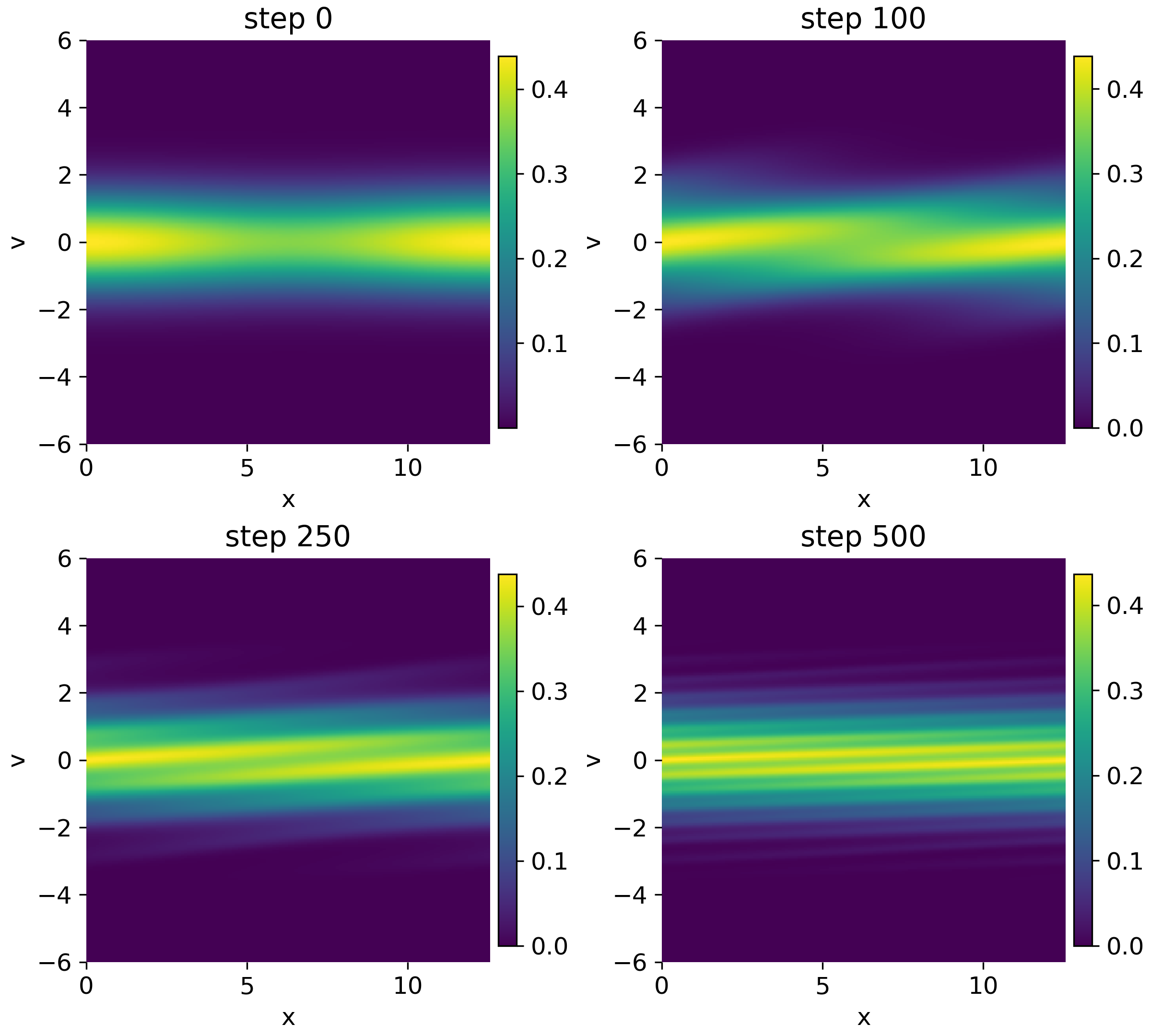
Snapshots of the phase-space distribution $(f(x,v,t))$ at increasing times. The bulk distribution remains Maxwellian while the perturbation is progressively sheared in phase space.

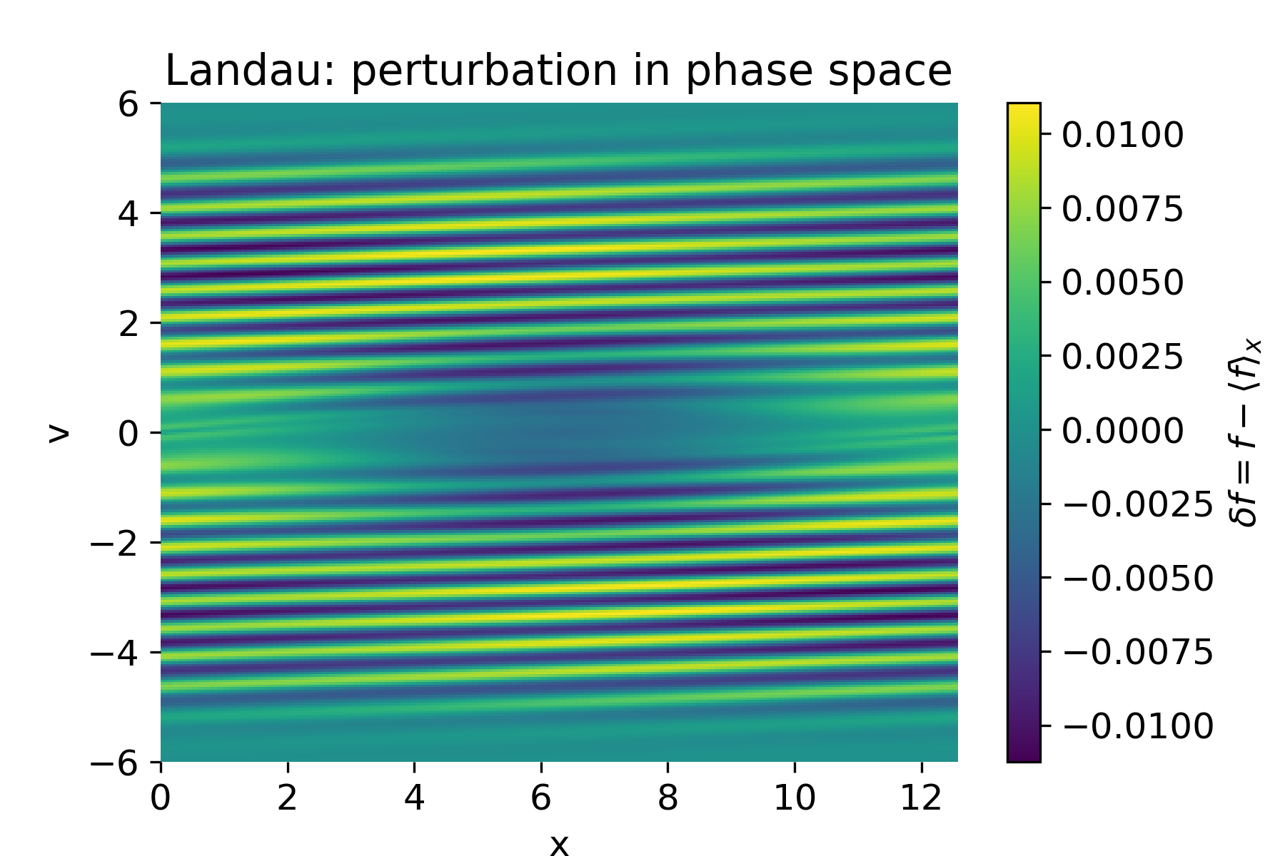
This interpretation is confirmed by the phase-space plots. While the spatially averaged distribution remains Maxwellian, the perturbation $\delta f = f - \langle f \rangle_x$ develops increasingly fine, slanted filaments in velocity space. These structures encode the damped wave energy and represent the kinetic memory of the initial perturbation.

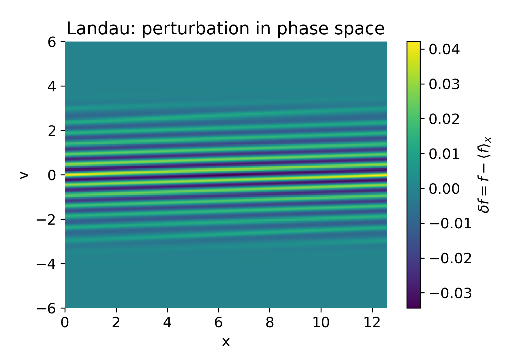
Perturbation distribution $(\delta f = f - \langle f \rangle_x)$ showing the development of fine velocity-space filaments. These structures represent the kinetic mechanism underlying Landau damping.

Two-stream instability mode (mode == "twostream")

In two-stream mode, the solver uses the same numerical scheme but a qualitatively different initial velocity distribution. Instead of a single Maxwellian, the plasma consists of two counter-streaming populations,

\[f(x,v,0) = \left[1 + \alpha \cos(kx)\right] \frac{1}{2}\left[f_M(v-u) + f_M(v+u)\right],\]

where (u) is the drift velocity of each beam. This distribution contains free energy in velocity space and is unstable to electrostatic perturbations.

As in the Landau case, the Vlasov equation is solved by phase-space advection and the electric field is obtained from Poisson’s equation. The difference in behavior arises entirely from the velocity-space structure of the initial condition.

Parameters and their physical meaning:

• alpha Amplitude of the initial spatial modulation. Larger values seed the instability more strongly and shorten the linear growth phase.
• k_mode Wave number of the perturbation. Only certain modes are unstable for given beam velocities; changing k_mode selects different instability branches.
• vt Thermal spread of each beam. Increasing vt broadens the velocity distributions and can partially stabilize the system by reducing velocity-space gradients.
• u Drift velocity of the two counter-streaming populations. Larger values increase the available free energy and typically lead to stronger and faster instability growth.

Numerical results and interpretation

The electric field energy initially oscillates but then grows as the instability extracts energy from the velocity distribution. This growth continues until nonlinear effects set in and particle trapping occurs. At that point, the field energy saturates and approaches a quasi-steady value.

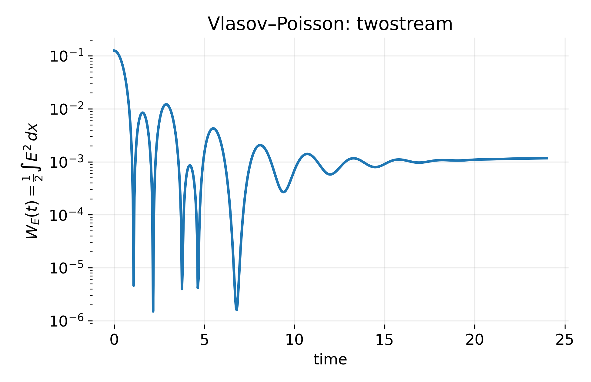
Electric field energy $(W_E(t))$ for the two-stream instability. After an initial transient, the field energy grows due to the extraction of free energy from the counter-streaming velocity distribution and eventually saturates due to nonlinear particle trapping.

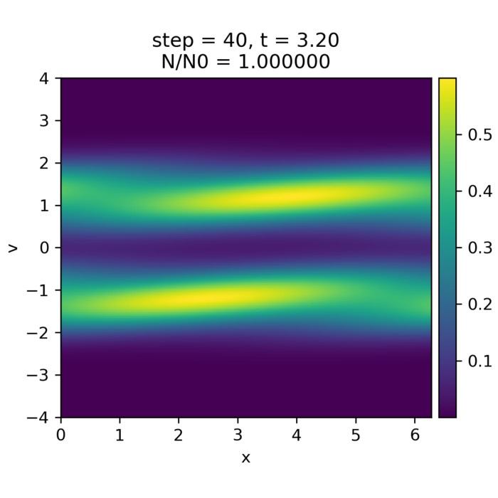
Phase-space snapshots show the characteristic deformation of the two beams. The initially narrow streams are bent and broadened by the self-generated electric field, leading to a partial flattening of the velocity distribution near resonant velocities. The perturbation $(\delta f)$ exhibits coherent, growing structures rather than the purely filamentary patterns seen in Landau damping.

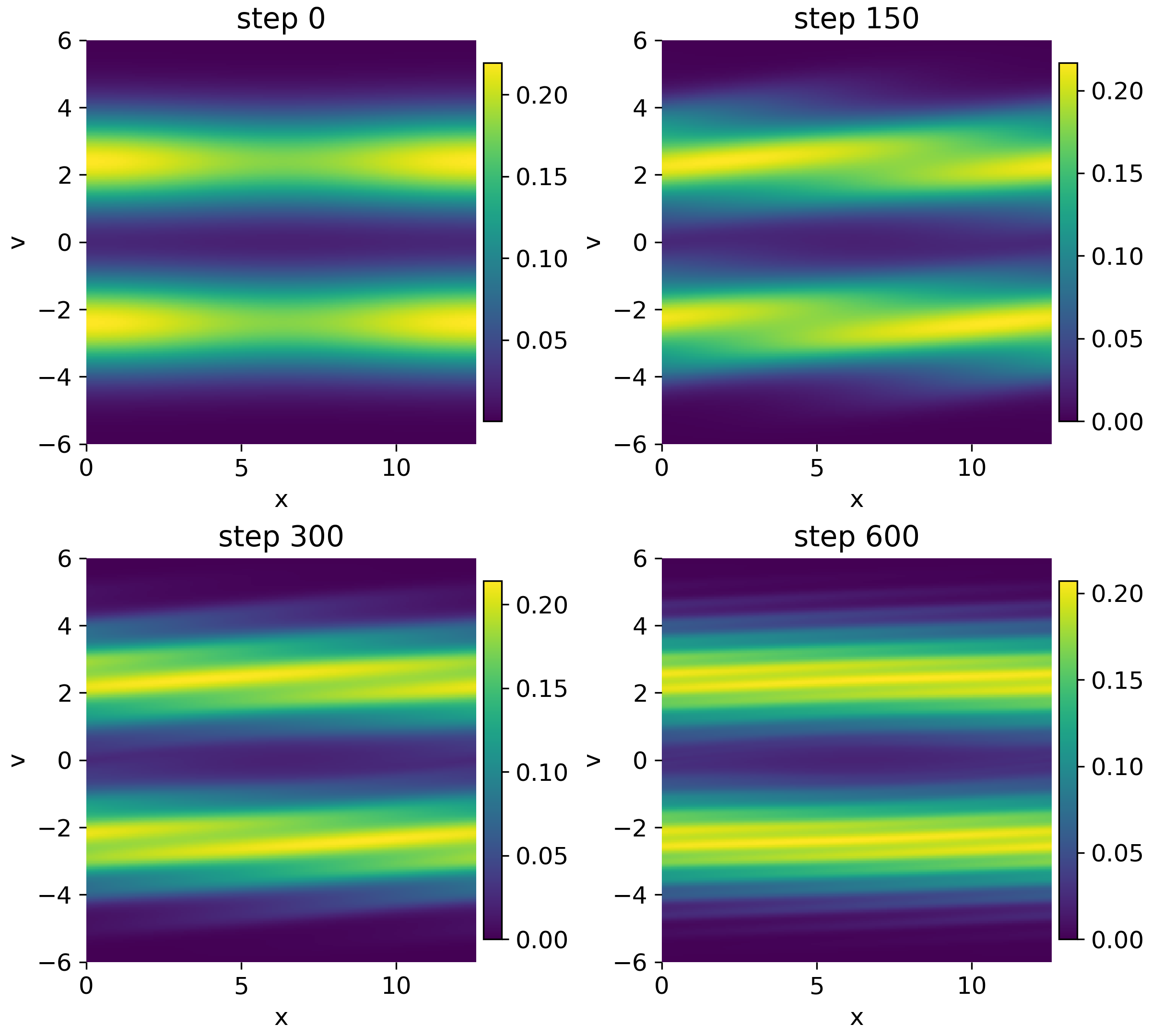
Phase-space evolution of $(f(x,v,t))$ showing the deformation and broadening of the two counter-streaming beams as the instability develops and saturates.

This behavior highlights the contrast between damping by phase mixing and genuine kinetic instability driven by velocity-space free energy.

Perturbation distribution $(\delta f)$ for the two-stream instability. Coherent structures grow in phase space, reflecting resonant wave–particle interaction and nonlinear saturation rather than simple phase mixing.

Scope and limitations of the numerical demonstration

The simulations presented here are intended as illustrative toy models. Finite velocity domains, limited resolution, and interpolation introduce numerical diffusion and eventual recurrence effects. Quantitative agreement with analytical growth or damping rates is not the goal. Instead, the emphasis lies on capturing the correct physical mechanisms and their phase-space signatures.

Within this scope, I hope the examples serve as concrete realizations of the abstract concepts introduced in kinetic plasma theory: Liouville’s theorem, collisionless phase-space advection, and the central role of velocity-space structure in plasma dynamics.

Update and code availability: This post and its accompanying Python code were originally drafted in 2020 and archived during the migration of this website to Jekyll and Markdown. In January 2026, I substantially revised and extended the code. The updated and cleaned-up implementation is now available in this new GitHub repositoryꜛ. Please feel free to experiment with it and to share any feedback or suggestions for further improvements.

References and further reading

• Wolfgang Baumjohann and Rudolf A. Treumann, Basic Space Plasma Physics, 1997, Imperial College Press, ISBN: 1-86094-079-X
• Treumann, R. A., Baumjohann, W., Advanced Space Plasma Physics, 1997, Imperial College Press, ISBN: 978-1-86094-026-2
• Donald A. Gurnett, Amitava Bhattacharjee, Introduction to plasma physics with space and laboratory applications, 2005, Cambridge University Press, ISBN: 978-7301245491
• Francis F. Chen, Introduction to plasma physics and controlled fusion, 2016, Springer, ISBN: 978-3319223087
• R. C. Davidson, Methods in nonlinear plasma theory, 1972, Academic Press, ISBN: 978-0122054501