What velocity moments miss: Core plus beam distributions

A central step in plasma physics is the reduction of the full kinetic description to a fluid or magnetohydrodynamic one. This reduction proceeds by taking velocity moments of the distribution function $f(\mathbf{x},\mathbf{v},t)$, yielding macroscopic quantities such as density, bulk velocity, and temperature. While this procedure is mathematically well defined, it is also inherently lossy: infinitely many different distribution functions can share the same low order moments.

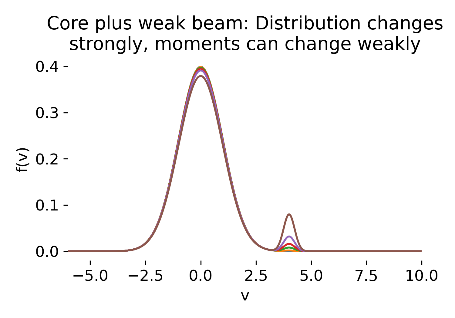Core plus weak beam velocity distribution $f(v)$ for increasing beam strength $\epsilon$. In this post, we explore how different initial velocity distributions lead to qualitatively distinct macroscopic dynamics, illustrating the inherently kinetic nature of these processes.

The purpose of this tutorial is to make this loss of information explicit and tangible. Rather than evolving a kinetic equation in time, we construct controlled families of velocity distributions and examine how strongly their kinetic structure can change while their lowest fluid moments remain nearly unchanged. This provides a minimal and concrete demonstration of why fluid closures can hide physically relevant kinetic effects, even in apparently simple situations.

The example is deliberately static and one-dimensional in velocity. Its role is conceptual rather than dynamical: To isolate the mapping from distribution functions to moments and to show how non thermal structure can be invisible to fluid variables.

Physical setup: Core plus weak beam

We consider a one dimensional velocity distribution composed of a dominant thermal core and a weak beam component,

\[f(v) = (1-\epsilon)\,f_{\text{core}}(v) + \epsilon\,f_{\text{beam}}(v),\]

where $0 \le \epsilon \ll 1$ controls the beam strength.

The core distribution is taken to be a Maxwellian centered at zero velocity,

\[f_{\text{core}}(v) = \frac{1}{\sqrt{2\pi v_{t}^{2}}} \exp\!\left(-\frac{v^{2}}{2 v_{t}^{2}}\right),\]

with thermal speed $v_t$.

The beam is represented by a narrower Maxwellian centered at a finite drift velocity $v_{\text{beam}}$,

\[f_{\text{beam}}(v) = \frac{1}{\sqrt{2\pi v_{b}^{2}}} \exp\!\left(-\frac{(v-v_{\text{beam}})^{2}}{2 v_{b}^{2}}\right),\]

with $v_b \ll v_t$.

Two configurations are studied:

• an asymmetric case with a single beam at $+v_{\text{beam}}$
• a symmetric case with two identical beams at $\pm v_{\text{beam}}$, each carrying half of the beam weight

In both cases, the total distribution is normalized such that the particle density remains constant as $\epsilon$ is varied.

Velocity moments

From each constructed distribution we compute the lowest velocity moments,

\[\begin{align} n &= \int f(v)\,dv, \\ u &= \frac{1}{n}\int v f(v)\,dv, \\ T &\propto \frac{1}{n}\int (v-u)^2 f(v)\,dv. \end{align}\]

These quantities correspond to the density, bulk velocity, and temperature that would be used in a fluid or MHD description. Higher order moments and the detailed shape of $f(v)$ are deliberately discarded.

Numerical realization

The distribution functions are evaluated on a sufficiently fine velocity grid, and all integrals are computed numerically using direct quadrature. The beam strength $\epsilon$ is varied over several orders of magnitude, from effectively zero to a few percent, while all other parameters are kept fixed.

The numerical experiment consists of:

• constructing $f(v)$ for different values of $\epsilon$
• visualizing the full velocity distributions
• zooming into the beam region to expose weak kinetic structure
• computing and plotting $n(\epsilon)$, $u(\epsilon)$, and $T(\epsilon)$

So, let’s begin with the necessary imports:

import numpy as np
import matplotlib.pyplot as plt

# remove spines right and top for better aesthetics:
plt.rcParams['axes.spines.right'] = False
plt.rcParams['axes.spines.top'] = False
plt.rcParams['axes.spines.left'] = False
plt.rcParams['axes.spines.bottom'] = False
plt.rcParams.update({'font.size': 12})

The first thing we need are functions that define the distributions (one for the Maxwellian, one for the core plus beam mixture):

# 1D Maxwellian:
def maxwell_1d(v, n=1.0, u=0.0, vt=1.0):
    """
    1D Maxwellian:
        f(v) = n / (sqrt(2*pi)*vt) * exp( - (v-u)^2 / (2 vt^2) )
    Here vt is the 1D thermal speed (standard deviation).
    """
    return n / (np.sqrt(2.0 * np.pi) * vt) * np.exp(-0.5 * ((v - u) / vt) ** 2)

# Mixture: core plus beam:
def core_plus_beam(v, eps=0.02, n=1.0, u_core=0.0, vt_core=1.0, u_beam=4.0, vt_beam=0.3):
    """
    Mixture model:
        f = (1-eps) f_core + eps f_beam
    Both components are normalized so that integral f dv = n.
    """
    f_core = maxwell_1d(v, n=n, u=u_core, vt=vt_core)
    f_beam = maxwell_1d(v, n=n, u=u_beam, vt=vt_beam)
    return (1.0 - eps) * f_core + eps * f_beam

Then, we need to compute the velocity moments from a given distribution:

def velocity_moments(v, f):
    """
    Compute density n, bulk velocity u, and 1D temperature-like variance T
    from velocity moments.

    n = ∫ f dv
    u = (1/n) ∫ v f dv
    T ~ (1/n) ∫ (v-u)^2 f dv

    Note:
    * In kinetic theory, pressure p = m ∫ (v-u)^2 f dv, and T = p/(n k_B).
      Here we return the variance sigma^2 = (1/n) ∫ (v-u)^2 f dv as a proxy for temperature.
    """
    dv = v[1] - v[0]
    n = np.sum(f) * dv
    u = np.sum(v * f) * dv / n
    var = np.sum(((v - u) ** 2) * f) * dv / n
    return n, u, var

Now we set up the parameters for the numerical experiment by defining the velocity grid, base distribution parameters, and the list of beam strengths to explore:

# velocity grid:
vmin, vmax = -10.0, 10.0
Nv = 40001  # large enough to resolve a narrow beam; reduce if needed for speed
v = np.linspace(vmin, vmax, Nv)

# base parameters:
params = dict(
    n=1.0,
    u_core=0.0,
    vt_core=1.0,
    u_beam=4.0,
    vt_beam=0.25)

# beam strengths to compare;
eps_list = [0.0, 1e-3, 5e-3, 1e-2, 2e-2, 5e-2]

To compute the distributions and their moments for each value of $\epsilon$, we use the following loop:

# compute distributions and moments:
moments = []
fs = []
for eps in eps_list:
    f = core_plus_beam(v, eps=eps, **params)
    n, u, Tvar = velocity_moments(v, f)
    moments.append((eps, n, u, Tvar))
    fs.append(f)
moments = np.array(moments, dtype=float)  

As diagnostics, we create three plots, which show

• the full velocity distributions for different $\epsilon$
• a zoom-in on the beam region
• the moments $n(\epsilon)$, $u(\epsilon)$, and $T(\epsilon)$ as functions of $\epsilon$

# plot 1: f(v) for different eps
plt.figure(figsize=(7, 4))
for f, eps in zip(fs, eps_list):
    plt.plot(v, f, label=f"eps = {eps:g}")
plt.xlim(-6, 10)
plt.xlabel("v")
plt.ylabel("f(v)")
plt.title("Core plus weak beam: Distribution changes\nstrongly, moments can change weakly")
plt.legend(frameon=False)
plt.tight_layout()
plt.savefig("velocity_distribution_vs_eps.png", dpi=300)
plt.close()

# plot 2: zoom-in on the beam region
plt.figure(figsize=(7, 4))
for f, eps in zip(fs, eps_list):
    plt.plot(v, f, label=f"eps = {eps:g}")
plt.xlim(1.5, 7.0)
plt.ylim(0, None)
plt.xlabel("v")
plt.ylabel("f(v)")
plt.title("Zoom near the beam: Small eps introduces clear\nkinetic structure")
plt.legend(frameon=False)
plt.tight_layout()
plt.savefig("velocity_distribution_zoom_vs_eps.png", dpi=300)
plt.close()

# plot 3: moments vs eps
eps = moments[:, 0]
n = moments[:, 1]
u = moments[:, 2]
Tvar = moments[:, 3]
fig = plt.figure(figsize=(7, 7))
ax1 = fig.add_subplot(311)
ax1.plot(eps, n, marker="o")
ax1.set_xlabel("eps")
ax1.set_ylabel("n")
ax1.set_title("Velocity moments vs beam strength eps")
ax1.grid(True, alpha=0.3)
ax2 = fig.add_subplot(312)
ax2.plot(eps, u, marker="o")
ax2.set_xlabel("eps")
ax2.set_ylabel("u")
ax2.grid(True, alpha=0.3)
ax3 = fig.add_subplot(313)
ax3.plot(eps, Tvar, marker="o")
ax3.set_xlabel("eps")
ax3.set_ylabel("T (variance)")
ax3.grid(True, alpha=0.3)
plt.tight_layout()
plt.savefig("velocity_moments_vs_eps.png", dpi=300)
plt.close()

Optionally, we can repeat the same analysis for the symmetric beam configuration:

def symmetric_beams(v, eps=0.02, n=1.0, u_core=0.0, vt_core=1.0, u_beam=4.0, vt_beam=0.25):
    """
    Symmetric two-beam mixture:
        f = (1-eps) f_core + (eps/2) f_beam(+u) + (eps/2) f_beam(-u)
    This keeps bulk velocity closer to zero while still adding strong kinetic structure.
    """
    f_core = maxwell_1d(v, n=n, u=u_core, vt=vt_core)
    f_bp = maxwell_1d(v, n=n, u=+u_beam, vt=vt_beam)
    f_bm = maxwell_1d(v, n=n, u=-u_beam, vt=vt_beam)
    return (1.0 - eps) * f_core + 0.5 * eps * f_bp + 0.5 * eps * f_bm

eps_list2 = [0.0, 1e-3, 5e-3, 1e-2, 2e-2, 5e-2]
moments2 = []
fs2 = []

for eps_ in eps_list2:
    f2 = symmetric_beams(v, eps=eps_, **params)
    n2, u2, T2 = velocity_moments(v, f2)
    moments2.append((eps_, n2, u2, T2))
    fs2.append(f2)

moments2 = np.array(moments2, dtype=float)

plt.figure(figsize=(7, 4))
for f2, eps_ in zip(fs2, eps_list2):
    plt.plot(v, f2, label=f"eps = {eps_:g}")
plt.xlim(-7, 7)
plt.xlabel("v")
plt.ylabel("f(v)")
plt.title("Symmetric weak beams: strong kinetic structure with u ~ 0")
plt.legend(frameon=False)
plt.tight_layout()
plt.savefig("symmetric_velocity_distribution_vs_eps.png", dpi=300)
plt.close()

fig = plt.figure(figsize=(7, 7))
ax1 = fig.add_subplot(311)
ax1.plot(moments2[:, 0], moments2[:, 1], marker="o")
ax1.set_xlabel("eps")
ax1.set_ylabel("n")
ax1.set_title("Moments vs eps (symmetric beams)")
ax1.grid(True, alpha=0.3)

ax2 = fig.add_subplot(312)
ax2.plot(moments2[:, 0], moments2[:, 2], marker="o")
ax2.set_xlabel("eps")
ax2.set_ylabel("u")
ax2.grid(True, alpha=0.3)

ax3 = fig.add_subplot(313)
ax3.plot(moments2[:, 0], moments2[:, 3], marker="o")
ax3.set_xlabel("eps")
ax3.set_ylabel("T (variance)")
ax3.grid(True, alpha=0.3)

plt.tight_layout()
plt.savefig("symmetric_velocity_moments_vs_eps.png", dpi=300)
plt.close()

Discussion of the results

In the following, we analyze the results of the numerical experiment for both the asymmetric and symmetric beam configurations.

Asymmetric beam: strong kinetic change, weak moment response

The velocity distribution $f(v)$ exhibits the most direct and informative change as the beam strength $\epsilon$ is increased. For $\epsilon = 0$, the distribution is a single Maxwellian centered at $v = 0$. As soon as $\epsilon > 0$, a secondary peak appears at $v \approx v_{\text{beam}}$. Its amplitude scales linearly with $\epsilon$, while its width is set by the beam thermal spread $v_b$.

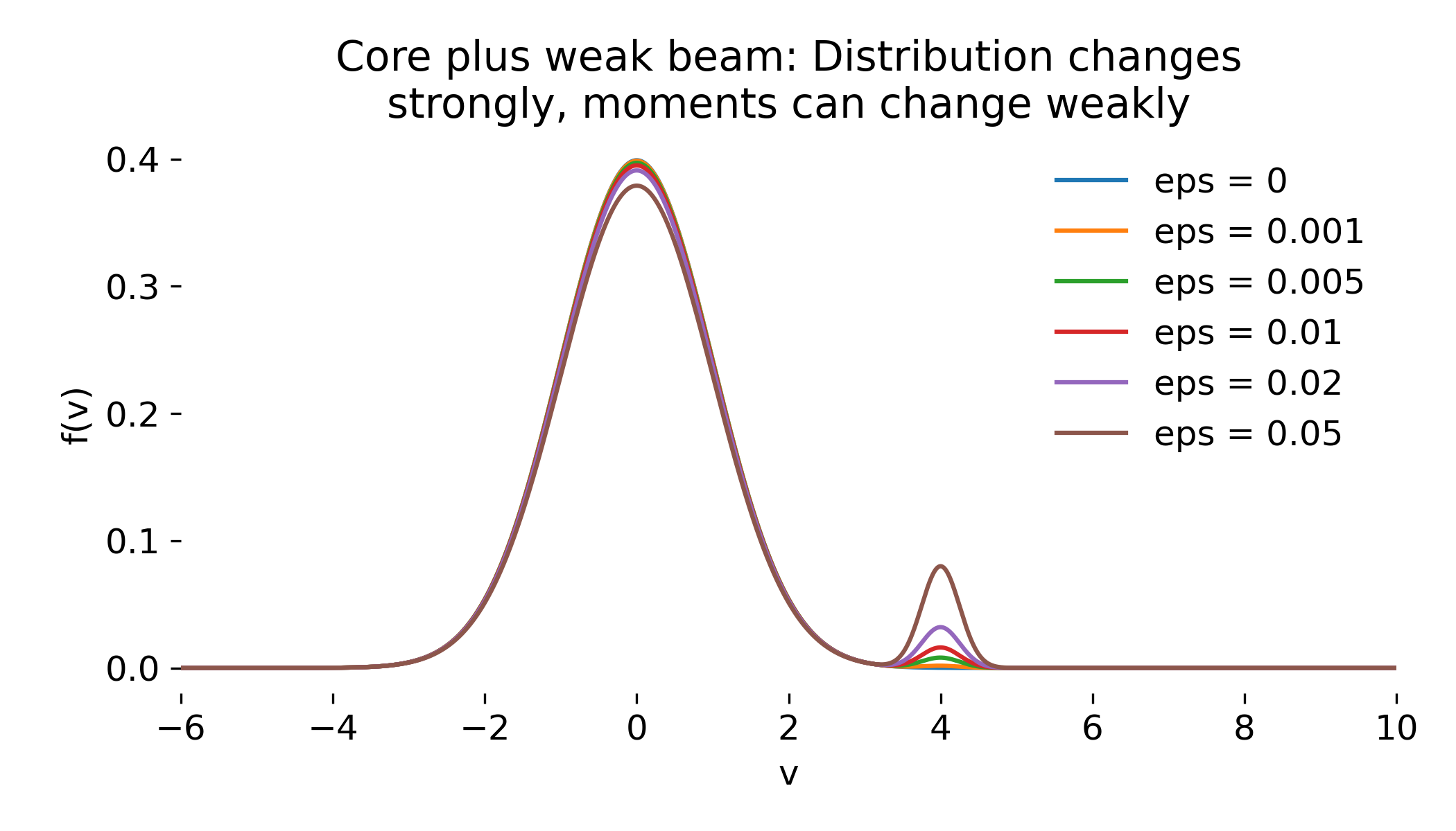
Core plus weak beam velocity distribution $f(v)$ for increasing beam strength $\epsilon$. Even a very small beam fraction introduces a distinct non thermal population at high velocity while the Maxwellian core remains dominant.

To make this beam more visible, we created a zoomed-in plot around $v_{\text{beam}}$. This zoom-in reveals that the beam is already well separated from the core in velocity space:

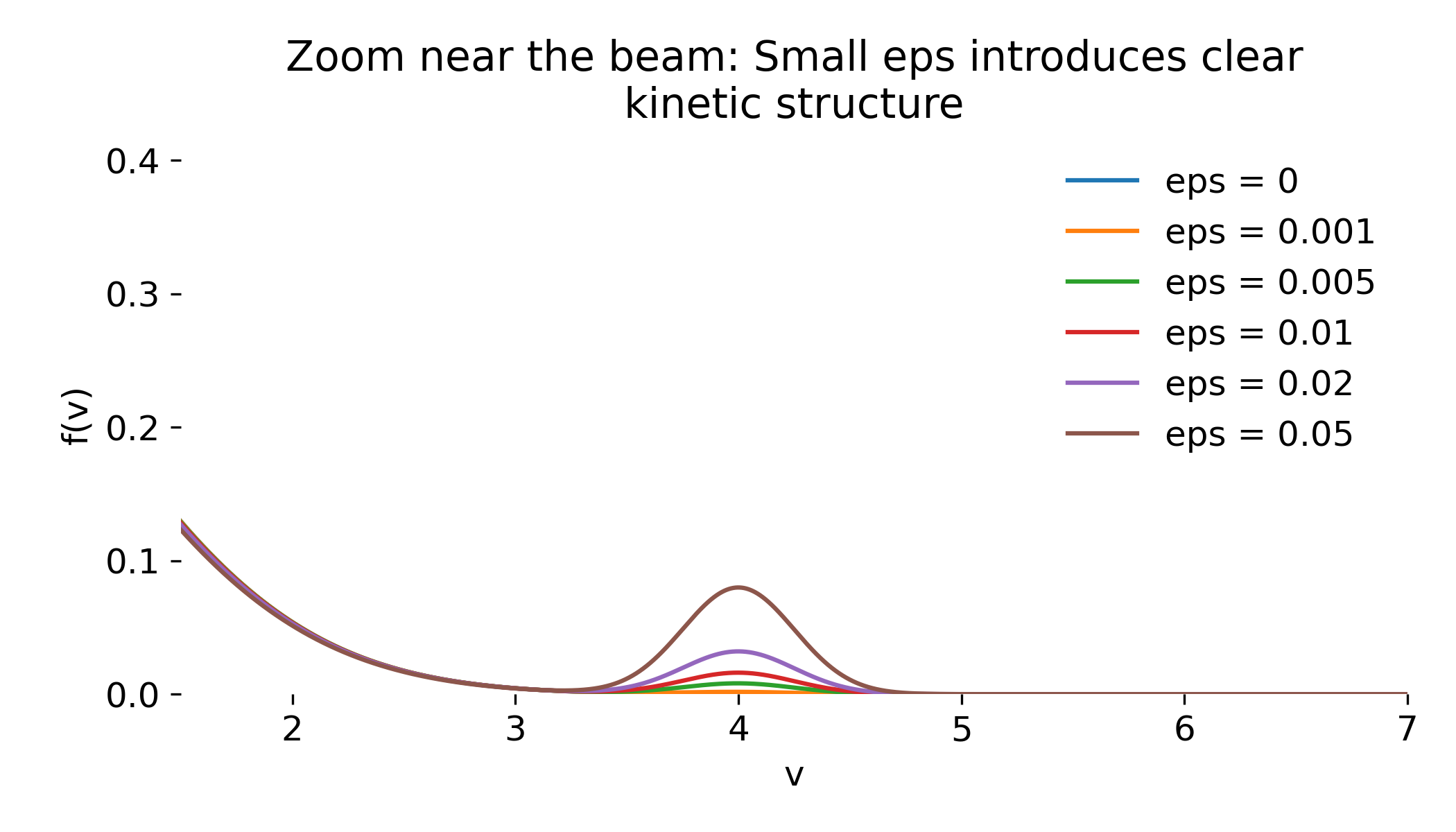
Zoom of the velocity distribution near the beam velocity, showing that small $\epsilon$ produces a clearly resolved kinetic feature that is hidden in the full range view.

Mathematically, this reflects the fact that $f(v)$ is a sum of distributions with disjoint support, even though one component carries only a small fraction of the total density.

The density moment

\[n(\epsilon) = \int f(v)\,dv\]

remains exactly constant by construction. This is reflected in the top panel of the plot below, where $n$ is independent of $\epsilon$ up to numerical precision.

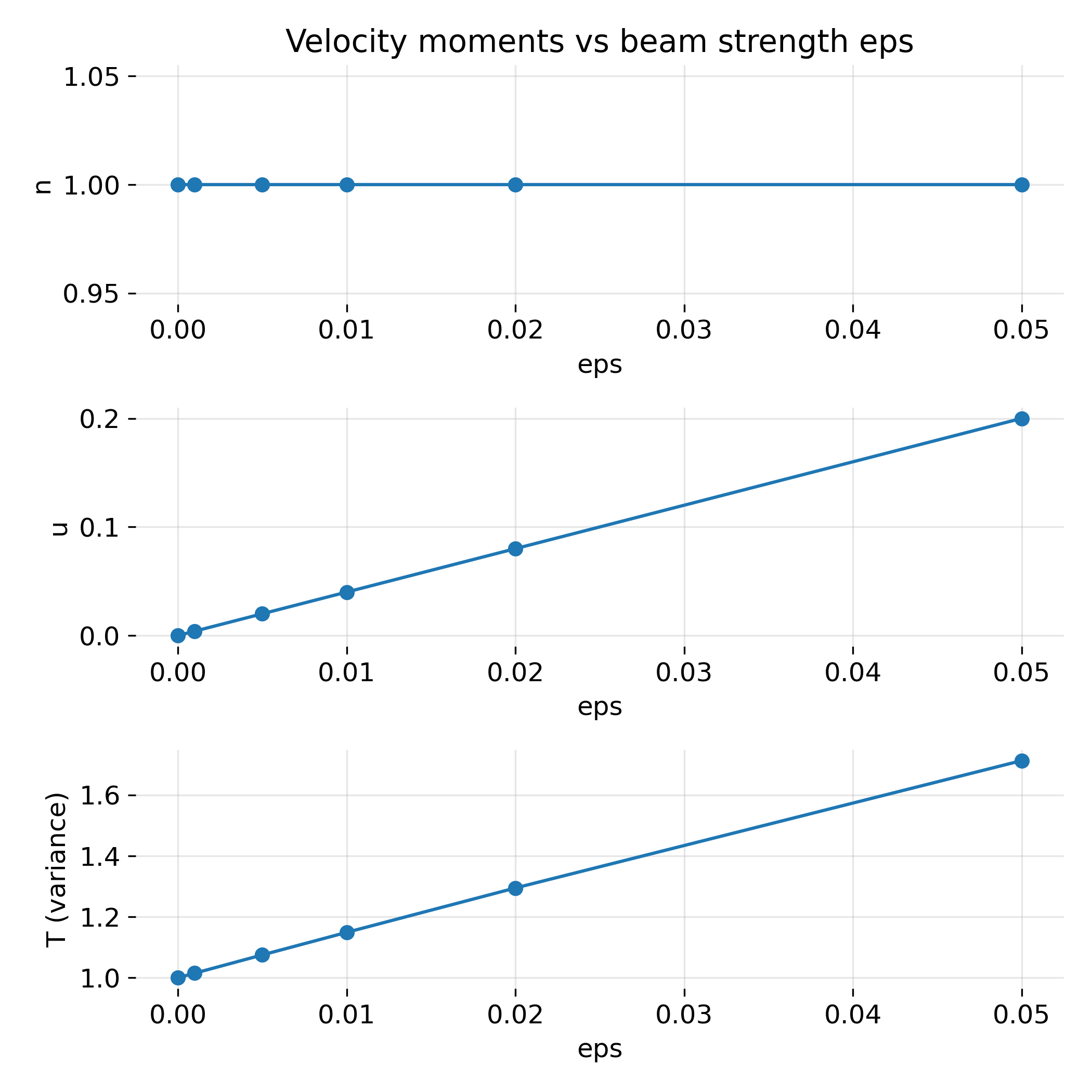
Top: Density $n$ as a function of beam strength $\epsilon$, demonstrating exact conservation of total particle number despite strong changes in $f(v)$. – Middle: Bulk velocity $u$ versus beam strength $\epsilon$, showing a linear but weak response compared to the beam speed itself. – Bottom: Temperature $T$ as a function of $\epsilon$, illustrating that strongly non Maxwellian distributions can appear only mildly hotter in a moment description.

The bulk velocity (plotted in the middle panel)

\[u(\epsilon) = \frac{1}{n}\int v f(v)\,dv\]

increases approximately linearly with $\epsilon$. This follows directly from the decomposition of $f(v)$: The core contributes zero net momentum, while the beam contributes a momentum proportional to $\epsilon v_{\text{beam}}$. As a result,

\[u(\epsilon) \approx \epsilon\,v_{\text{beam}}\]

for small $\epsilon$.

The temperature (plotted in the bottom panel)

\[T(\epsilon) \propto \frac{1}{n}\int (v-u)^2 f(v)\,dv\]

shows a smooth, monotonic increase with $\epsilon$. This increase reflects the additional kinetic energy carried by the beam, but does not encode where in velocity space this energy resides.

Taken together, these plots show that a strong qualitative change in $f(v)$ corresponds only to weak, smooth variations in the lowest moments. From a fluid perspective, the plasma appears only slightly drifting and moderately hotter, while kinetically it contains a distinct fast population.

Symmetric beams: Kinetic structure without bulk flow

The symmetric beam configuration sharpens this point further. The velocity distribution now consists of a central Maxwellian core plus two symmetric beam components at $v = \pm v_{\text{beam}}$. As $\epsilon$ increases, the two non thermal peaks become clearly visible in $f(v)$, while the core remains essentially unchanged:

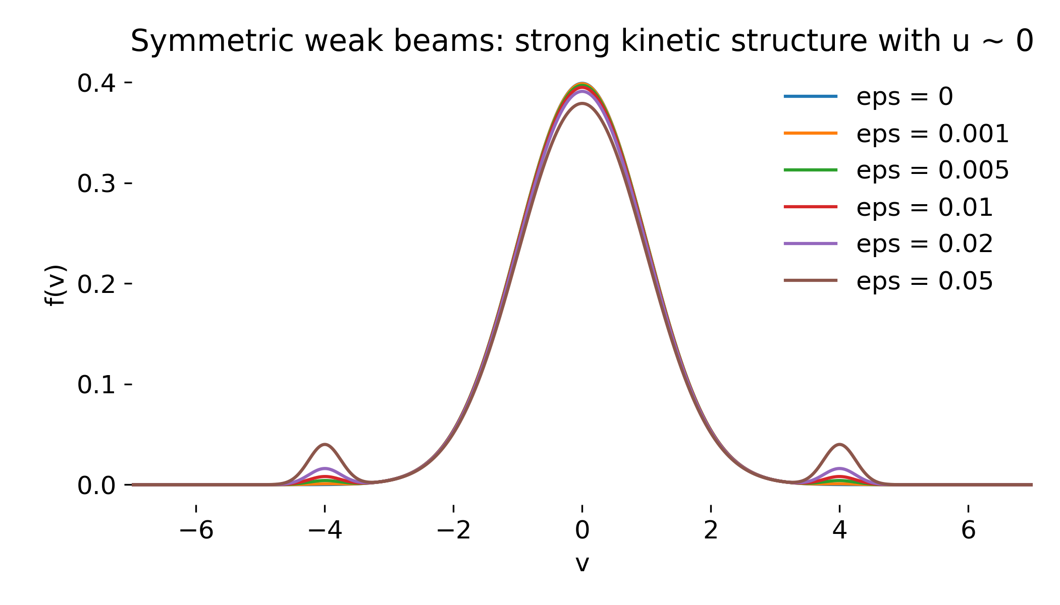
Velocity distributions with symmetric counter streaming beams. Two distinct non thermal populations develop while the core Maxwellian remains nearly unchanged.

Despite this pronounced kinetic structure, the bulk velocity

\[u(\epsilon) = \frac{1}{n}\int v f(v)\,dv\]

remains zero for all $\epsilon$. This follows directly from symmetry: the momentum contributions of the two beams cancel exactly.

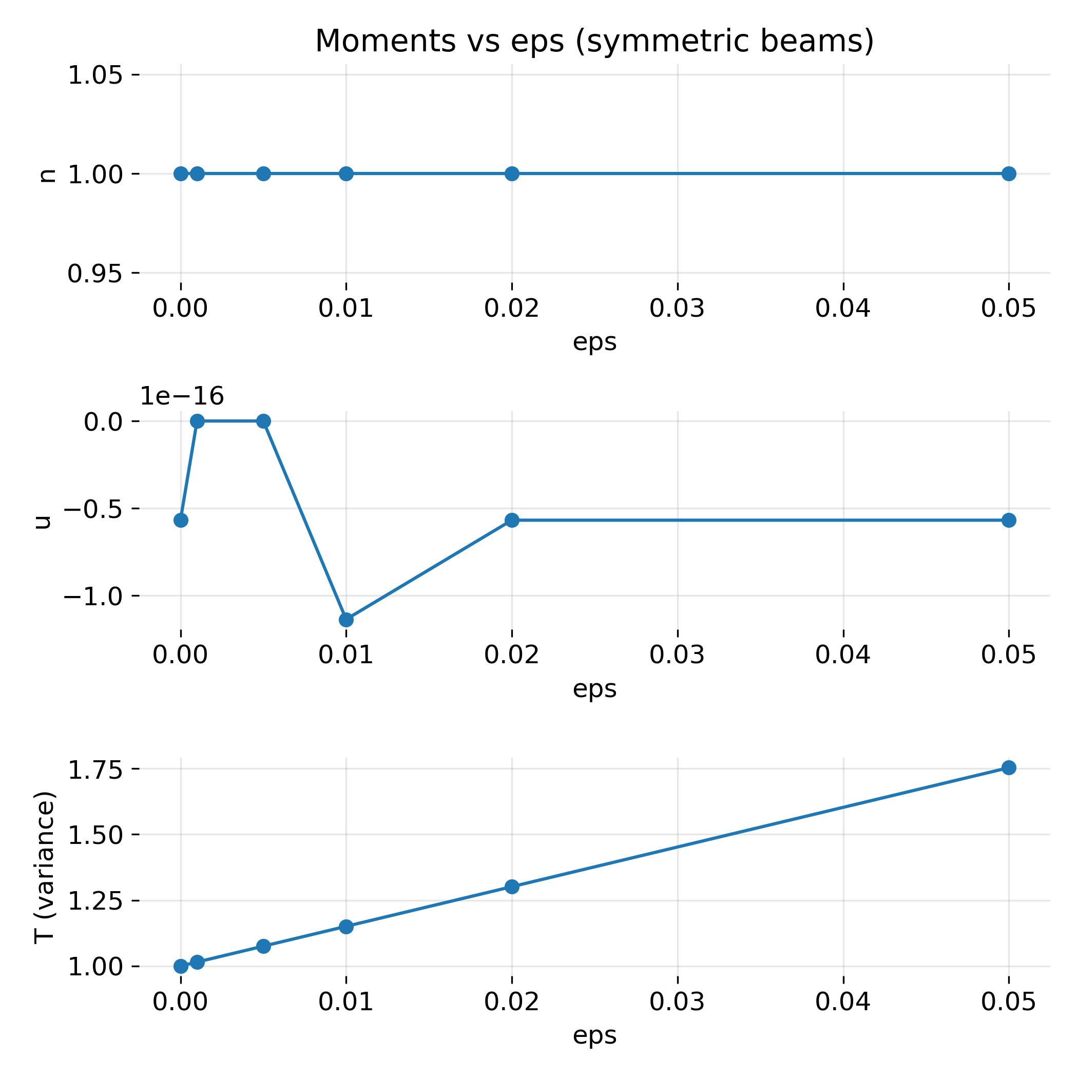
Top: Density $n$ remains constant by construction for all $\epsilon$. – Middle: Bulk velocity $u$ remains zero for all $\epsilon$ due to symmetry, despite strong kinetic structure in $f(v)$. – Bottom: Temperature $T$ versus $\epsilon$ for symmetric beams. The moment responds to added energy but does not reflect the existence of counter streaming populations.

The density again remains constant by construction. Only the temperature responds to the presence of the beams. As in the asymmetric case, $T(\epsilon)$ increases smoothly with $\epsilon$, reflecting the added kinetic energy.

This case demonstrates explicitly that the absence of bulk flow does not imply the absence of directed particle motion. A plasma can be strongly non Maxwellian while having vanishing first moment.

Physical interpretation and implications

These results make the loss of information in moment based descriptions explicit. The mapping

\[f(v) \;\longrightarrow\; \{n, u, T\}\]

is many to one: Qualitatively different distributions produce nearly identical moments. In the present examples, sharply localized beam populations remain almost invisible to the lowest order moments.

This loss is not merely quantitative but structural. Features such as multiple velocity populations, phase space gaps, or narrow beams are precisely the ingredients that control kinetic processes like Landau damping, wave particle resonance, and beam driven instabilities. None of these can be inferred from $n$, $u$, and $T$ alone.

From this perspective, fluid and MHD models should be understood as controlled projections of kinetic theory rather than as complete descriptions. They capture averaged dynamics while systematically discarding information that may become dynamically decisive in weakly collisional or collisionless plasmas.

The present static construction isolates this point in its simplest possible form. Without invoking any time evolution or instability, it shows directly and quantitatively what is lost when velocity space structure is reduced to a small set of moments.

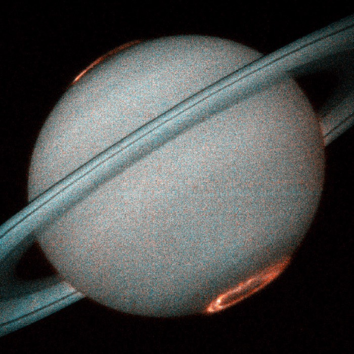
Relevance for space plasmas

The core-plus-beam distributions constructed here are not artificial corner cases, but closely resemble velocity distributions routinely observed in space plasmas. In the solar wind, in planetary magnetospheres, and in auroral acceleration regions, particle distributions often consist of a dominant thermal core accompanied by weak beams or high-energy tails. Examples include electron strahl populations in the solar wind, ion beams upstream of collisionless shocks, and counter-streaming particle populations along magnetic field lines.

In many of these environments, the beam fraction $\epsilon$ is small in terms of particle number, yet dynamically significant. As demonstrated by the present example, such beams can remain almost invisible at the level of fluid moments while fundamentally altering the kinetic behavior of the plasma. Wave–particle resonances, Landau damping, and beam-driven instabilities depend sensitively on the detailed shape of $f(v)$ rather than on its lowest moments. A plasma that appears only weakly drifting and moderately heated in an MHD description may therefore be strongly unstable or dissipative when viewed kinetically.

This is particularly relevant in weakly collisional space plasmas, where the assumption of rapid relaxation toward a Maxwellian is not justified. In such regimes, velocity-space structure can persist over macroscopic distances and timescales, and moment-based closures necessarily obscure the physical mechanisms that govern energy transfer, wave generation, and particle acceleration. The present static construction isolates this point in its simplest form, but its implications extend directly to real space physics observations.

Conclusion

By constructing simple core plus beam distributions and examining their velocity moments, we have shown explicitly how strong kinetic structure can coexist with nearly unchanged fluid variables. This example clarifies, in the most direct possible way, what is lost when passing from a kinetic to a fluid description.

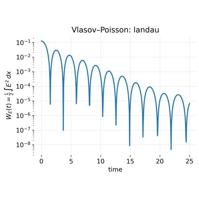
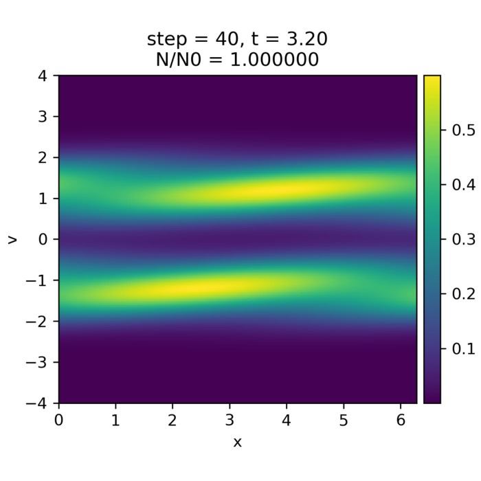
The result provides a conceptual bridge to fully kinetic simulations, such as those based on the Vlasov equation, where the full phase space structure is retained and allowed to evolve dynamically.

Update and code availability: This post and its accompanying Python code were originally drafted in 2020 and archived during the migration of this website to Jekyll and Markdown. In January 2026, I substantially revised and extended the code. The updated and cleaned-up implementation is now available in this new GitHub repositoryꜛ. Please feel free to experiment with it and to share any feedback or suggestions for further improvements.

References and further reading

• Wolfgang Baumjohann and Rudolf A. Treumann, Basic Space Plasma Physics, 1997, Imperial College Press, ISBN: 1-86094-079-X
• Treumann, R. A., Baumjohann, W., Advanced Space Plasma Physics, 1997, Imperial College Press, ISBN: 978-1-86094-026-2
• Donald A. Gurnett, Amitava Bhattacharjee, Introduction to plasma physics with space and laboratory applications, 2005, Cambridge University Press, ISBN: 978-7301245491
• Francis F. Chen, Introduction to plasma physics and controlled fusion, 2016, Springer, ISBN: 978-3319223087
• R. C. Davidson, Methods in nonlinear plasma theory, 1972, Academic Press, ISBN: 978-0122054501