Krook collision operator as velocity-space relaxation

September 18, 2020 January 23, 2026 11 minute read see also comments

Collisions play a fundamentally different role in kinetic plasma theory than transport or collective field dynamics. While the Vlasov equation describes conservative phase space advection, collision operators introduce irreversibility by driving the distribution function toward a prescribed equilibrium.

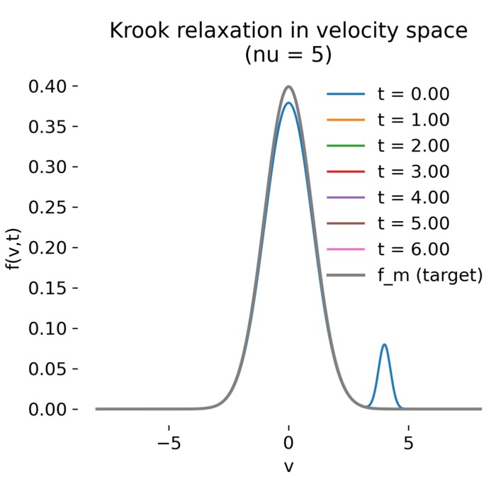
Krook collision operator relaxation snapshots with collision frequency $\nu = 5$. In this post, we explore the Krook collision operator as a minimal model for velocity-space relaxation in kinetic plasma theory.

In this tutorial, a minimal collisional model is considered: the Krook collision operator. Rather than attempting to reproduce microscopic Coulomb collisions, the Krook operator provides a controlled and analytically tractable description of velocity-space relaxation. Its purpose is conceptual clarity rather than realism.

The model isolates the meaning of a collision term by stripping away spatial dependence, self-consistent fields, and nonlinear feedback. What remains is a clean demonstration of how collisions act as a relaxation process in velocity space and how macroscopic moments respond.

Mathematical model

The system is zero-dimensional in space and one-dimensional in velocity. The kinetic equation reads

\[\partial_t f(v,t) = \nu\,[f_m(v) - f(v,t)],\]

where

$f(v,t)$ is the evolving velocity distribution,
$f_m(v)$ is a fixed Maxwellian target distribution,
$\nu$ is the collision frequency.

This equation has the exact solution

\[f(v,t) = f_m(v) + \bigl[f_0(v) - f_m(v)\bigr] e^{-\nu t},\]

where $f_0(v)$ is the initial distribution.

The dynamics is linear, local in velocity space, and purely dissipative. No transport, phase space mixing, or wave-particle interaction is present.

Numerical implementation

The numerical realization follows directly from the analytic solution.

Velocity grid and distributions

A uniform velocity grid $v \in [v_{\min}, v_{\max}]$ is defined with sufficiently high resolution to resolve both a thermal core and a narrow beam component. The initial distribution $f_0(v)$ is chosen as a non-Maxwellian core-plus-beam mixture, while the target distribution $f_m(v)$ is a Maxwellian with the same density.

Time evolution

Rather than integrating the differential equation explicitly, the analytic solution is evaluated at discrete times $t$. This avoids numerical stiffness issues for large $\nu$ and ensures that the relaxation dynamics is represented exactly.

Multiple collision frequencies $\nu$ are explored to demonstrate how the relaxation time scale depends on collisionality.

Diagnostics

The following quantities are computed as functions of time:

the $L^2$ distance to equilibrium,
\[\| f(t) - f_m \|_2 = \left(\int |f(v,t) - f_m(v)|^2\,dv\right)^{1/2},\]
the velocity moments
\[\begin{aligned} n(t) &= \int f(v,t)\,dv \\ u(t) &= \frac{1}{n}\int v f(v,t)\,dv \\ T(t) &\propto \frac{1}{n}\int (v-u)^2 f(v,t)\,dv \end{aligned}\]
snapshots of $f(v,t)$ at selected times.

Python code

Let’s start by importing necessary libraries and setting up plotting aesthetics:

import numpy as np
import matplotlib.pyplot as plt

# remove spines right and top for better aesthetics:
plt.rcParams['axes.spines.right'] = False
plt.rcParams['axes.spines.top'] = False
plt.rcParams['axes.spines.left'] = False
plt.rcParams['axes.spines.bottom'] = False
plt.rcParams.update({'font.size': 12})

Next, we need to define functions for the distributions, i.e., the Maxwellian and the core-plus-beam mixture:

def maxwell_1d(v, n=1.0, u=0.0, vt=1.0):
    return n / (np.sqrt(2.0 * np.pi) * vt) * np.exp(-0.5 * ((v - u) / vt) ** 2)


def core_plus_beam(v, eps=0.05, n=1.0, u_core=0.0, vt_core=1.0, u_beam=4.0, vt_beam=0.3):
    f_core = maxwell_1d(v, n=n, u=u_core, vt=vt_core)
    f_beam = maxwell_1d(v, n=n, u=u_beam, vt=vt_beam)
    return (1.0 - eps) * f_core + eps * f_beam

We also need utility functions for normalization,

def normalize_pdf(v, f):
    """
    Normalize f(v) such that ∫ f dv = 1 (or desired n if you rescale later).
    """
    Z = np.trapezoid(f, v)
    if Z <= 0 or not np.isfinite(Z):
        raise ValueError("Normalization failed.")
    return f / Z

and moment calculation:

def velocity_moments(v, f):
    """
    Compute n, u, variance (temperature proxy) for 1D distributions.
        n = ∫ f dv
        u = (1/n) ∫ v f dv
        var = (1/n) ∫ (v-u)^2 f dv
    """
    n = np.trapezoid(f, v)
    u = np.trapezoid(v * f, v) / n
    var = np.trapezoid(((v - u) ** 2) * f, v) / n
    return n, u, var

Now we implement the Krook relaxation function:

def krook_exact(f0, fm, nu, t):
    """
    Exact solution at time t:
        f(t) = fm + (f0 - fm) exp(-nu t)
    """
    return fm + (f0 - fm) * np.exp(-nu * t)

and the Euler time-stepping as an optional numerical check:

def krook_euler(f0, fm, nu, t_grid):
    f = f0.copy()
    out = [f.copy()]
    for i in range(1, len(t_grid)):
        dt = t_grid[i] - t_grid[i - 1]
        f = f + dt * nu * (fm - f)
        out.append(f.copy())
    return np.array(out)

Now we set up the simulation parameters:

# velocity grid:
vmin, vmax = -8.0, 8.0
Nv = 4000
v = np.linspace(vmin, vmax, Nv)

# target Maxwellian fm(v):
# choose an equilibrium state you want the collisions to enforce.
# Here: zero drift, vt=1.
fm = maxwell_1d(v, n=1.0, u=0.0, vt=1.0)
fm = normalize_pdf(v, fm)

# initial non-Maxwellian f0(v):
# Here: weak beam added to a core, then normalized.
f0 = core_plus_beam(v, eps=0.05, n=1.0, u_core=0.0, vt_core=1.0, u_beam=4.0, vt_beam=0.25)
f0 = normalize_pdf(v, f0)

# collision frequencies to compare:
nu_list = [0.2, 1.0, 5.0]

# time axis for plotting:
tmax = 6.0
Nt = 7
t_samples = np.linspace(0.0, tmax, Nt)

# for moment relaxation curves:
t_curve = np.linspace(0.0, tmax, 300)

A first analysis step is to visualize the initial and target distributions:

# plot 1: snapshots in time for each nu:
for nu in nu_list:
    plt.figure(figsize=(7.2, 4.6))
    for t in t_samples:
        ft = krook_exact(f0, fm, nu=nu, t=t)
        plt.plot(v, ft, label=f"t = {t:.2f}")
    plt.plot(v, fm, linewidth=2.0, label="f_m (target)")
    plt.xlabel("v")
    plt.ylabel("f(v,t)")
    plt.title(f"Krook relaxation in velocity space (nu = {nu:g})")
    plt.legend(frameon=False)
    plt.tight_layout()
    plt.savefig(f"krook_relaxation_snapshots_nu_{nu:g}.png", dpi=300)
    plt.close()

The next step is to track the relaxation of velocity moments over time:

# plot 2: relaxation of moments vs time (for each nu):
n_m, u_m, var_m = velocity_moments(v, fm)

plt.figure(figsize=(7.2, 7.2))
ax1 = plt.subplot(311)
ax2 = plt.subplot(312)
ax3 = plt.subplot(313)

for nu in nu_list:
    n_list = []
    u_list = []
    var_list = []
    for t in t_curve:
        ft = krook_exact(f0, fm, nu=nu, t=t)
        n_t, u_t, var_t = velocity_moments(v, ft)
        n_list.append(n_t)
        u_list.append(u_t)
        var_list.append(var_t)

    ax1.plot(t_curve, n_list, label=f"nu = {nu:g}")
    ax2.plot(t_curve, u_list, label=f"nu = {nu:g}")
    ax3.plot(t_curve, var_list, label=f"nu = {nu:g}")

ax1.axhline(n_m, linestyle="--", label="target")
ax2.axhline(u_m, linestyle="--")
ax3.axhline(var_m, linestyle="--")

ax1.set_ylabel("n")
ax2.set_ylabel("u")
ax3.set_ylabel("var ~ T")
ax3.set_xlabel("t")
ax1.set_title("Relaxation of velocity moments under Krook operator")
ax1.legend(frameon=False)
ax1.grid(True, alpha=0.3)
ax2.grid(True, alpha=0.3)
ax3.grid(True, alpha=0.3)
plt.tight_layout()
plt.savefig("krook_relaxation_moments.png", dpi=300)
plt.close()

A final diagnostic is the $L^2$ distance to equilibrium as a function of time:

# plot 3: L2 distance to equilibrium vs time:
plt.figure(figsize=(7.2, 4.6))
for nu in nu_list:
    dist = []
    for t in t_curve:
        ft = krook_exact(f0, fm, nu=nu, t=t)
        dist.append(np.sqrt(np.trapezoid((ft - fm) ** 2, v)))
    plt.semilogy(t_curve, dist, label=f"nu = {nu:g}")
plt.xlabel("t")
plt.ylabel(r"$||f - f_m||_2$")
plt.title("Krook relaxation: distance to equilibrium")
plt.legend(frameon=False)
plt.grid(True, which="both", alpha=0.3)
plt.tight_layout()
plt.savefig("krook_relaxation_distance.png", dpi=300)
plt.close()

Discussion of the results

In the following, we go through the main results of the simulation and interpret their physical meaning.

Distance to equilibrium

The first diagnostic we discuss (plot 3) tracks the norm $| f(t) - f_m |_2$ as a function of time for several collision frequencies $\nu$.

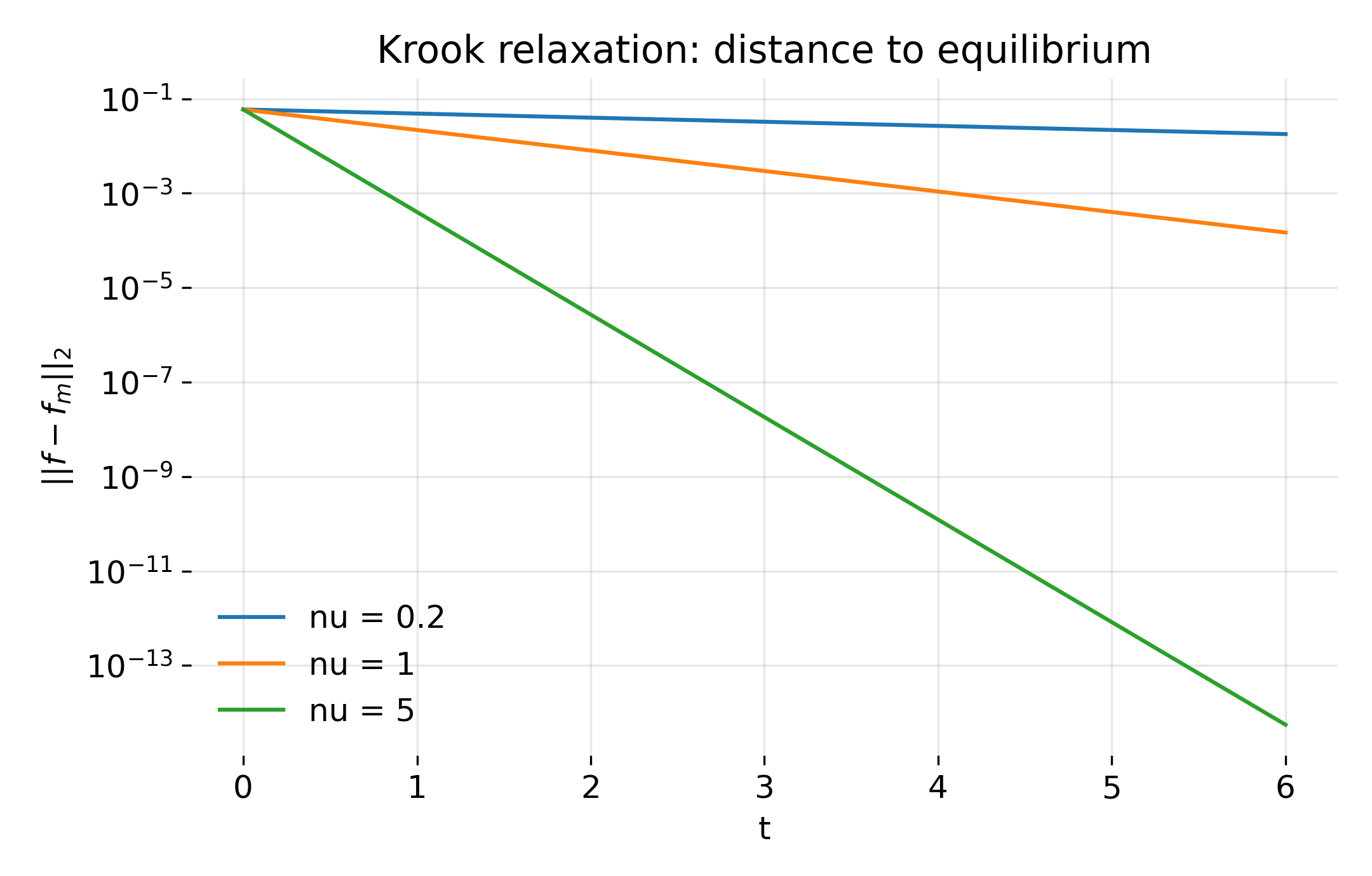
Exponential decay of the $L^2$ distance between the distribution function and the target Maxwellian under the Krook collision operator. Different collision frequencies $\nu$ produce straight lines on a logarithmic scale, demonstrating pure exponential relaxation with rate $\nu$.

The result is unambiguous: The distance decays exactly as $e^{-\nu t}$. Larger $\nu$ leads to faster relaxation, with no transient behavior or oscillations. This plot directly visualizes what a collision frequency means in kinetic theory: It sets a global relaxation rate in function space.

Relaxation of velocity moments

The second diagnostic shows (plot 2) the time evolution of density $n(t)$, bulk velocity $u(t)$, and temperature $T(t)$:

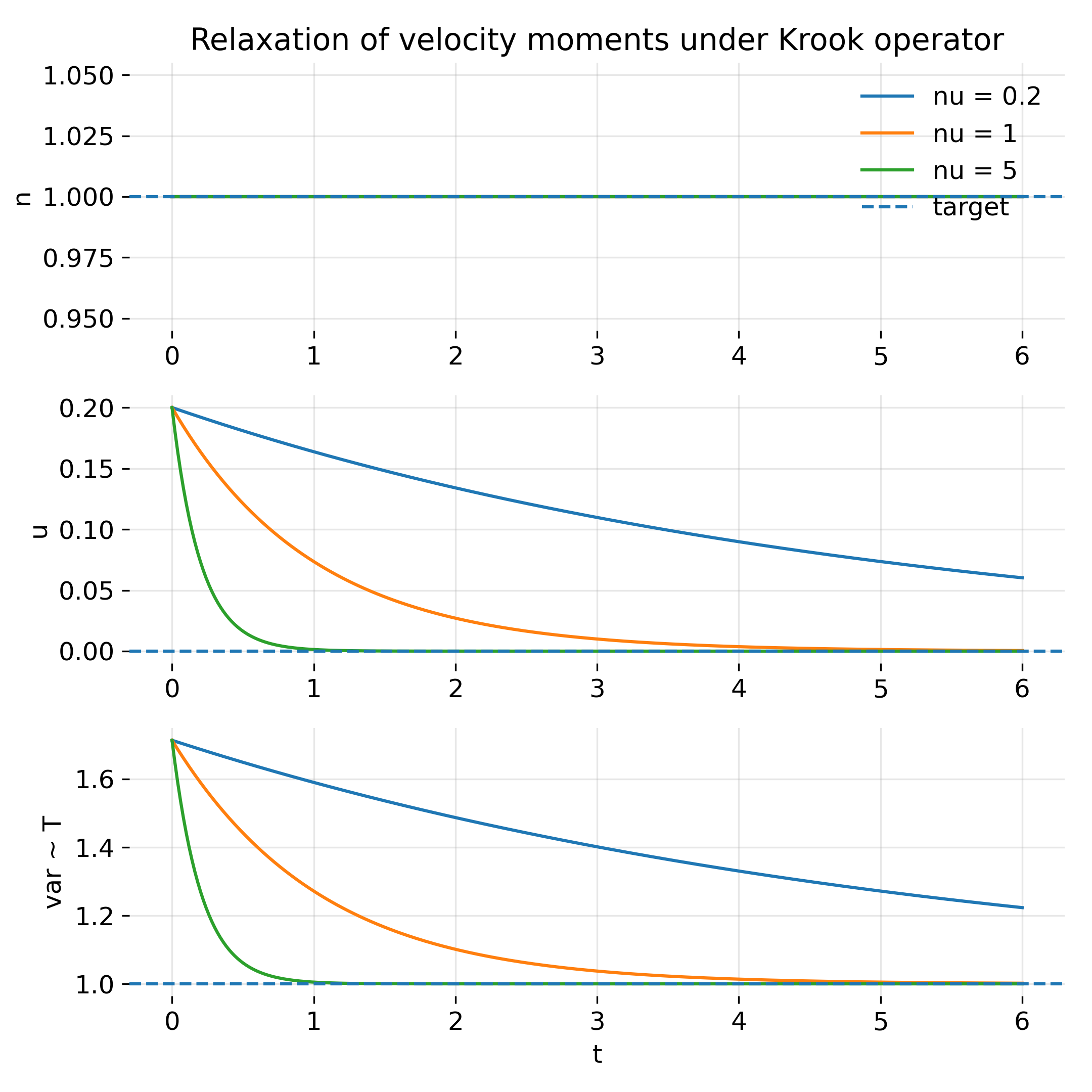
Time evolution of density, bulk velocity, and temperature under the Krook collision operator for different collision frequencies. Density remains constant by construction, while velocity and temperature relax exponentially toward their equilibrium values with rate $\nu$.

Several important points emerge:

Density is conserved exactly, because both $f_0$ and $f_m$ are normalized identically.
Bulk velocity relaxes exponentially to zero.
Temperature relaxes exponentially to the target value.

All moments relax on the same timescale $\nu^{-1}$. There is no hierarchy of relaxation rates and no coupling between moments beyond the trivial exponential decay.

Velocity-space relaxation for strong collisions

The velocity-space snapshots for large collision frequency illustrate rapid equilibration (plot 1):

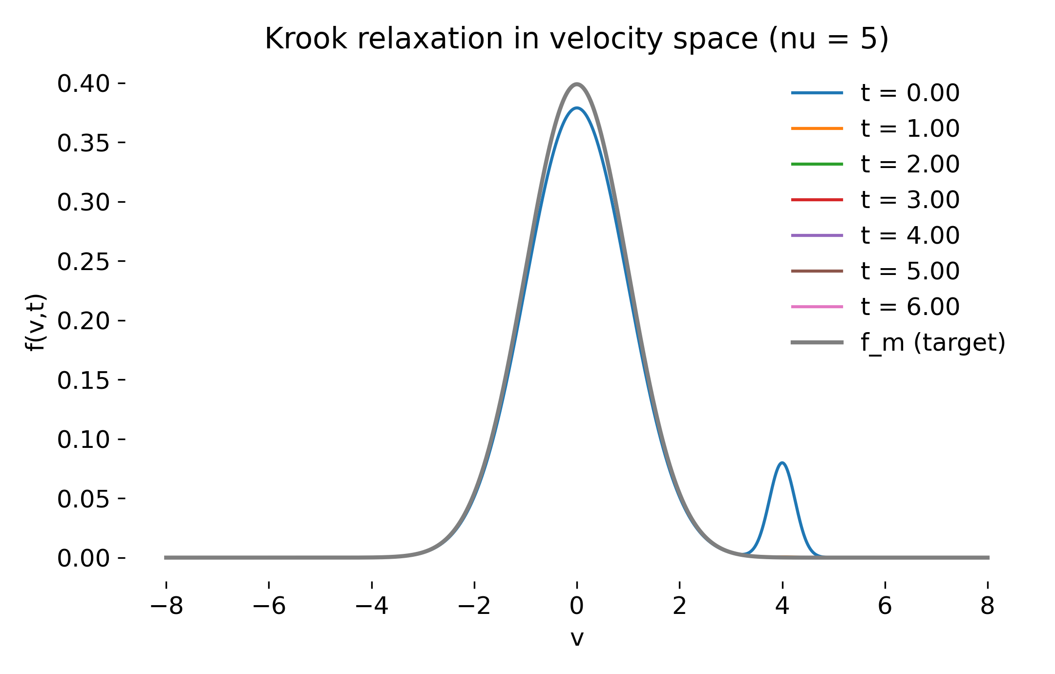
$Velocity-space snapshots for strong collisions ($\nu=5$).$
Velocity-space snapshots for strong collisions ($\nu=5$). A non-Maxwellian initial distribution relaxes rapidly toward the target Maxwellian, with the beam component disappearing on a timescale $\nu^{-1}$.

Here, the beam is erased almost immediately. The distribution closely matches the Maxwellian after only a short time, reflecting the dominance of collisional relaxation over kinetic structure.

Intermediate collision regime

For moderate collision frequencies, the relaxation is slower but qualitatively identical.

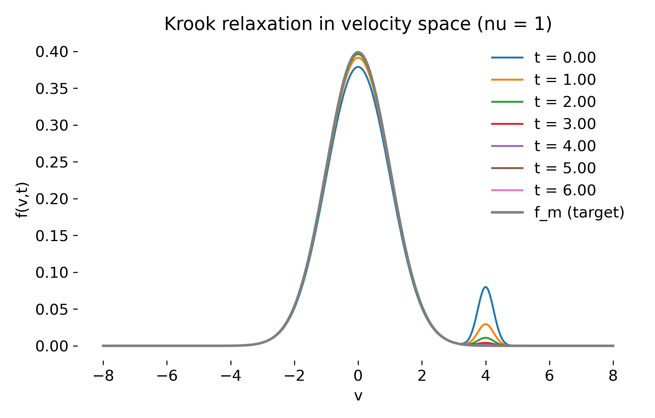
$Velocity-space snapshots for intermediate collisionality ($\nu=1$).$
Velocity-space snapshots for intermediate collisionality ($\nu=1$). The non-Maxwellian beam decays smoothly, and the distribution approaches the Maxwellian over several collision times.

The decay remains purely exponential. No distortion, filamentation, or redistribution in velocity space occurs.

Weakly collisional regime

Finally, weak collisions highlight the long-lived nature of non-Maxwellian features.

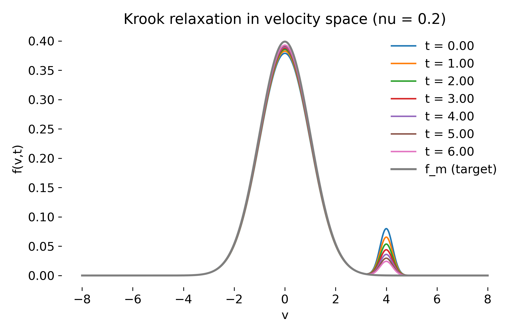
$Velocity-space snapshots for weak collisions ($\nu=0.2$).$
Velocity-space snapshots for weak collisions ($\nu=0.2$). Non-thermal features persist for long times, even though the distribution relaxes asymptotically toward the Maxwellian.

This regime is particularly relevant for collisionless plasmas: Kinetic structures can survive for times comparable to or longer than other dynamical timescales, even when a finite collisional relaxation mechanism is present.

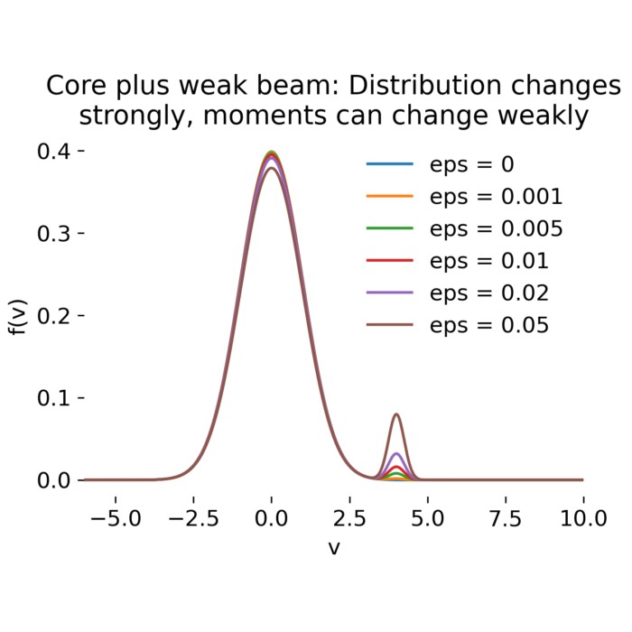
It is worth comparing these weak-collision snapshots with the static core-plus-weak-beam distributions discussed earlier:

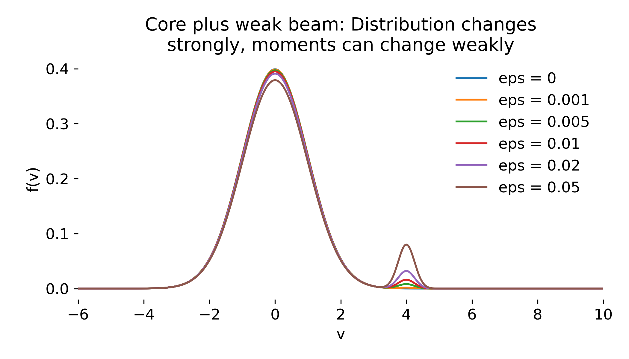
$Core plus weak beam velocity distribution $f(v)$ for increasing beam strength $\epsilon$.$
Core plus weak beam velocity distribution $f(v)$ for increasing beam strength $\epsilon$ from our post on velocity moments. For small collision frequencies, the Krook relaxation snapshots closely resemble these static mixtures, because the distribution remains close to its initial condition for times $t \ll \nu^{-1}$.

For small collision frequencies, the velocity-space structure at intermediate times closely resembles a superposition of a Maxwellian core and a weak suprathermal beam. This similarity is not a dynamical coincidence but a direct consequence of the chosen initial condition and the exponential relaxation law of the Krook operator. In both cases, the bulk of the distribution is dominated by the thermal core, while a small fraction of particles occupies a dynamically distinct region of velocity space.

The crucial difference is that, in the present case, the beam-like feature is not stationary but decays exponentially according to

\[f(v,t)=f_m(v)+\bigl(f_0(v)-f_m(v)\bigr)e^{-\nu t}.\]

For sufficiently small $\nu$, this relaxation timescale can be long compared to other physical processes, allowing non-Maxwellian features to persist and remain physically relevant even in formally collisional systems.

Physical interpretation and relevance for space physics

The Krook operator is not a microscopic model of Coulomb collisions. Instead, it represents an idealized relaxation mechanism that projects the distribution function onto a prescribed equilibrium. Its role is therefore not to reproduce detailed collisional physics, but to provide a controlled reference for how velocity-space structure would decay if collisions acted as homogeneous exponential relaxation.

This perspective connects directly to our earlier core-plus-weak-beam example. There, non-thermal velocity-space structure was introduced by construction and shown to be largely invisible to low-order moments. In the present Krook model, the same type of structure is deliberately used as an initial condition, allowing its collisional decay to be studied in isolation. For small collision frequencies, the distribution at intermediate times closely resembles a Maxwellian core plus a weak suprathermal beam. The similarity is therefore conceptual rather than emergent: In both situations, a small fraction of particles occupies a dynamically distinct region of velocity space while contributing little to the bulk moments.

The crucial difference is temporal. In the Krook model, the beam-like feature is not stationary but relaxes exponentially on the timescale $\nu^{-1}$. When $\nu$ is small, this relaxation time can be long compared to other dynamical processes, allowing non-Maxwellian structure to persist and remain physically relevant even in formally collisional systems. Weak collisionality therefore does not imply rapid equilibration in practice.

In space plasmas, true collisional frequencies are often extremely small. The solar wind, planetary magnetospheres, and the heliosheath are typically weakly collisional or effectively collisionless. In such environments:

Non-Maxwellian distributions are common.
Beams, plateaus, and anisotropies persist.
Relaxation is often dominated by wave–particle interactions rather than binary collisions.

From this viewpoint, the Krook operator provides a conceptual baseline rather than a realistic model. It answers the question: what would collisions do if they acted as simple, spatially homogeneous velocity-space relaxation? Real space plasmas deviate from this idealized picture in precisely the ways that make kinetic physics essential. Long-lived velocity-space structure, hidden from fluid moments and only weakly affected by collisions, is not an exception but a defining feature of collisionless plasma environments.

Conclusion

In this post, we have isolated the physical meaning of a collision term by studying the Krook operator in its simplest possible setting. The results show that:

Collisions act as exponential relaxation in velocity space.
All moments relax on the same timescale.
Non-Maxwellian structure is erased without transport, mixing, or nonlinear effects.

While the Krook operator is not a realistic collision model, it serves as a valuable conceptual baseline. By contrasting its behavior with collisionless Vlasov dynamics and more sophisticated collisional operators, we can gain a clearer understanding of what is retained and what is lost in different kinetic descriptions. This insight is particularly relevant for space physics, where weak collisionality allows non-Maxwellian features to persist and play a crucial role in plasma dynamics.

Update and code availability: This post and its accompanying Python code were originally drafted in 2020 and archived during the migration of this website to Jekyll and Markdown. In January 2026, I substantially revised and extended the code. The updated and cleaned-up implementation is now available in this new GitHub repositoryꜛ. Please feel free to experiment with it and to share any feedback or suggestions for further improvements.

References and further reading

Wolfgang Baumjohann and Rudolf A. Treumann, Basic Space Plasma Physics, 1997, Imperial College Press, ISBN: 1-86094-079-X
Treumann, R. A., Baumjohann, W., Advanced Space Plasma Physics, 1997, Imperial College Press, ISBN: 978-1-86094-026-2
Donald A. Gurnett, Amitava Bhattacharjee, Introduction to plasma physics with space and laboratory applications, 2005, Cambridge University Press, ISBN: 978-7301245491
Francis F. Chen, Introduction to plasma physics and controlled fusion, 2016, Springer, ISBN: 978-3319223087
R. C. Davidson, Methods in nonlinear plasma theory, 1972, Academic Press, ISBN: 978-0122054501