Particle-in-Cell methods in kinetic plasma simulations

Plasma physics is inherently multiscale. Collective electromagnetic fields evolve on macroscopic length and time scales, while the underlying charge carriers follow microscopic trajectories governed by the Lorentz force. Many plasma phenomena of interest, from kinetic instabilities to wave–particle interactions, cannot be described consistently by fluid models alone, yet are too complex to be treated analytically at the level of individual particles. The Particle-in-Cell (PIC) method was developed precisely to bridge this gap. It combines a kinetic description of charged particles with a self-consistent solution of the electromagnetic fields they generate, providing a numerical framework that retains microscopic physics while remaining computationally tractable.

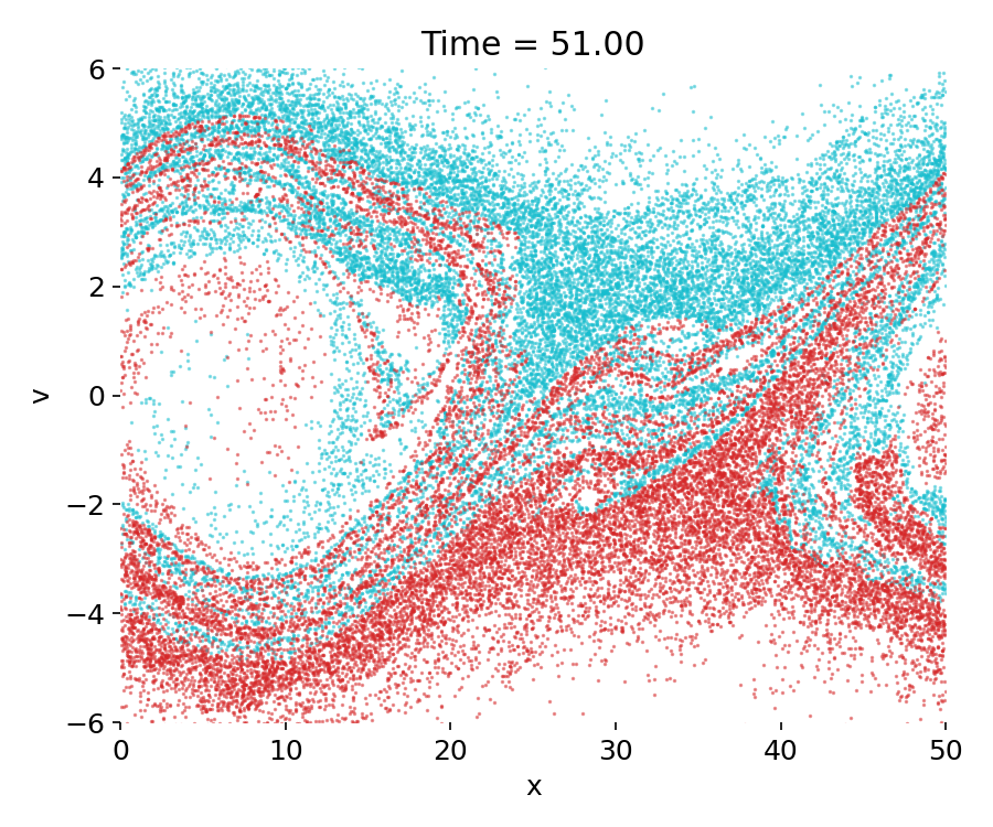
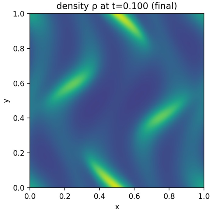
Particle-in-Cell simulation of electron dynamics in a plasma. The image shows a snapshot of electron macroparticles (colored dots) moving in self-consistent electric and magnetic fields (background color map and arrows). The PIC method tracks individual particle trajectories while solving Maxwell’s equations on a spatial grid, capturing kinetic effects such as trapping, wave–particle interactions, and non-Maxwellian distributions. The code is based on Philip Moczꜛ’s PIC Python implementationꜛ, which we will explore in more detail below.

In space physics, PIC methods play a particularly important role. Collisionless plasmas dominate the heliosphere, planetary magnetospheres, and much of astrophysical plasma environments. Phenomena such as magnetic reconnection, collisionless shocks, auroral acceleration, wave–particle scattering, and kinetic instabilities all require a description beyond magnetohydrodynamics. PIC simulations therefore form a central methodological pillar of modern space plasma research, complementing both fluid models and spacecraft observations.

What is Particle-in-Cell and how does it work?

The Particle-in-Cell method is a hybrid numerical scheme. The plasma distribution function is represented by a finite number of computational particles, often called macroparticles, which move continuously in phase space. The electromagnetic fields, in contrast, are represented on a fixed spatial grid. Particles interact with the fields through the Lorentz force, while the fields are updated from the charge and current densities deposited by the particles onto the grid.

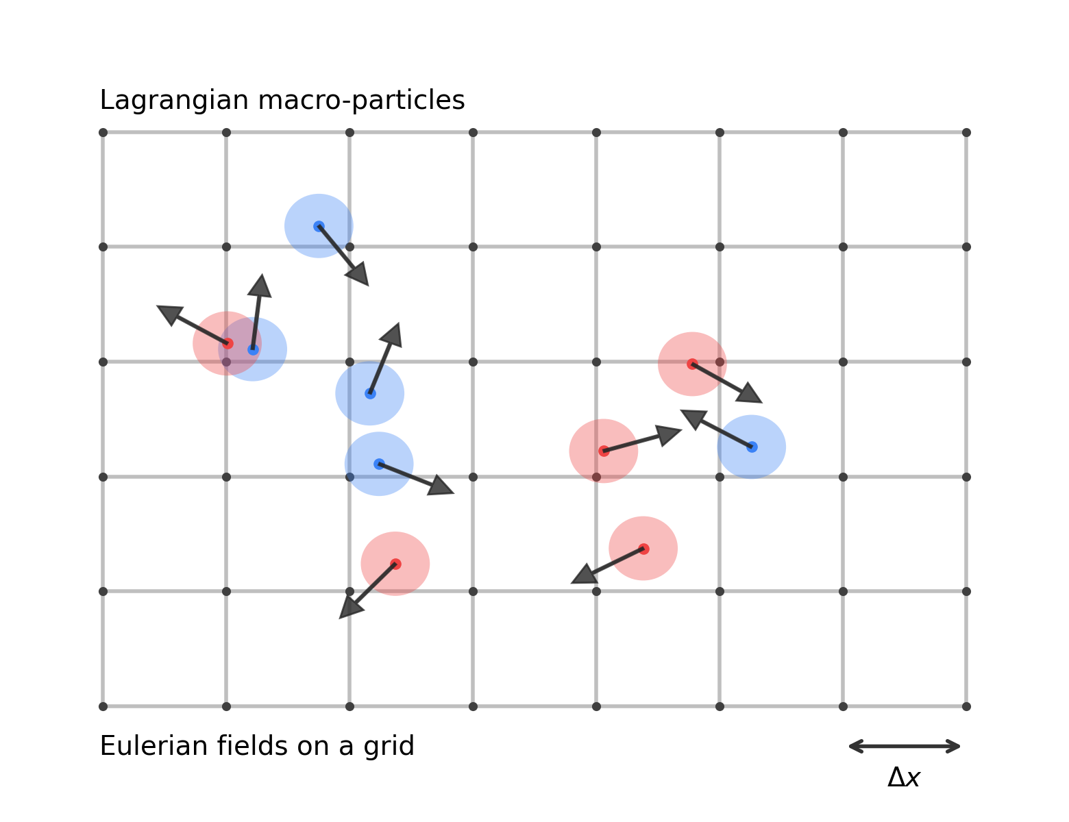
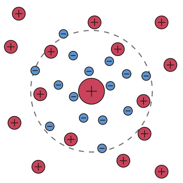
Eulerian–Lagrangian split in the Particle-in-Cell method. The PIC method represents plasma dynamics using two complementary descriptions. Macroparticles follow continuous trajectories in phase space (Lagrangian description) and carry charge and velocity information, indicated here by arrows. Different colors indicate different particle species or populations (for example electrons and ions, or counter-streaming beams), as commonly used in PIC simulations. Electromagnetic fields are defined on a fixed spatial grid (Eulerian description). The grid spacing $\Delta x$ sets the spatial resolution of the field solve, while particles move freely across cell boundaries. Coupling between particles and fields is achieved through charge and current deposition to the grid and field interpolation back to particle positions.

This separation of roles is essential. Tracking fields on a grid avoids the prohibitive cost of computing pairwise Coulomb interactions between particles. At the same time, following particle trajectories allows one to capture kinetic effects such as velocity space structure, trapping, and non-Maxwellian distributions, which are inaccessible to fluid closures.

A single PIC time step typically consists of four conceptually distinct stages:

1. particle-to-grid projection of charge and current,
2. field solve on the grid,
3. interpolation of the fields back to particle positions, and
4. advancement of particle positions and velocities.

In PIC terminology, these steps are often summarized as deposit (project particle charge/current to the grid), field solve (update $\mathbf{E}$ and $\mathbf{B}$ on the grid from Poisson or Maxwell), gather (interpolate the grid fields back to particle positions), and push (advance particles under the Lorentz force using a pusher such as Boris or, in electrostatic form, leapfrog). The algorithm is explicit in time in its simplest form and can be extended to electromagnetic, relativistic, or implicit variants.

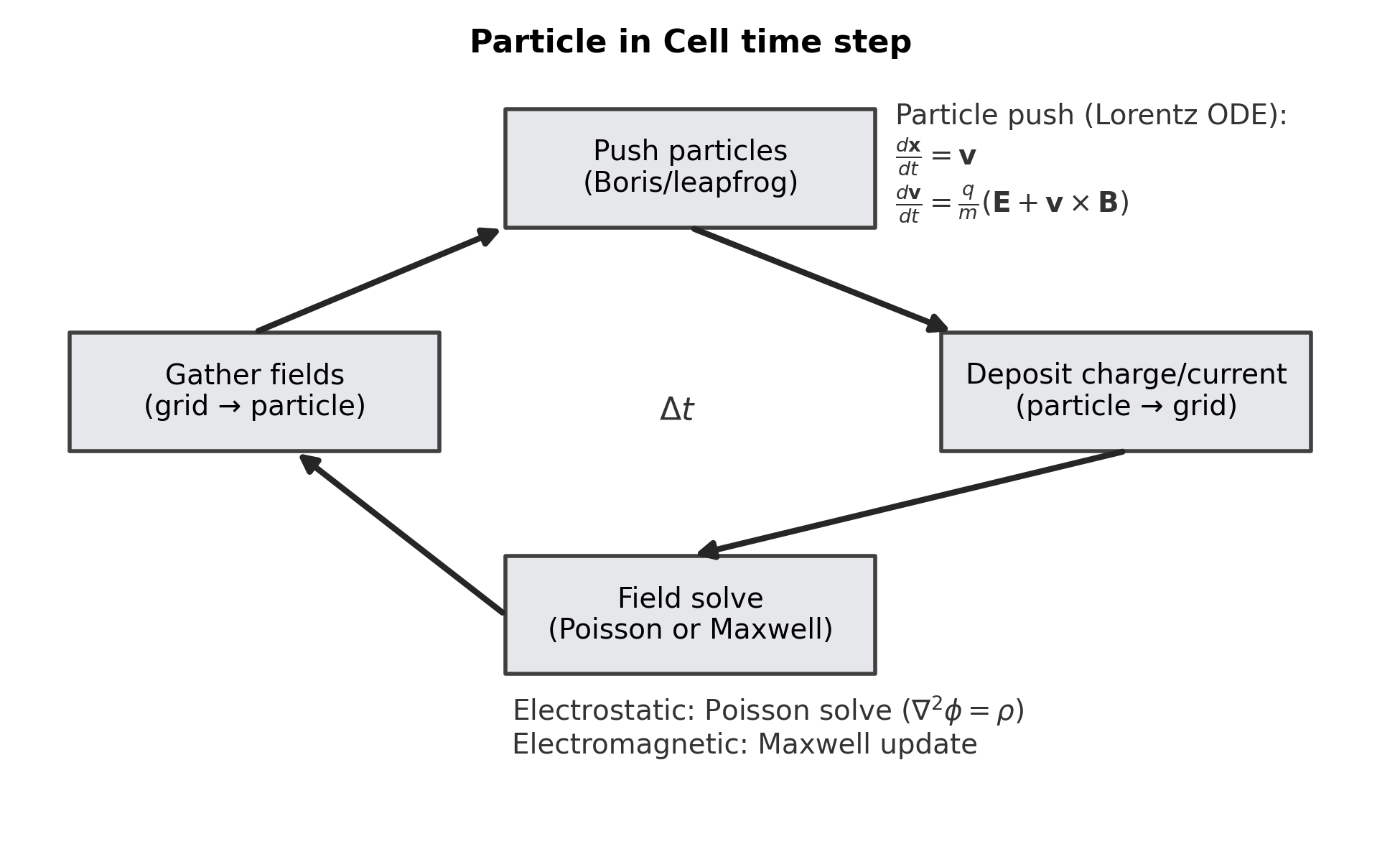
Particle-in-Cell time step and algorithmic loop. A single PIC time step consists of four tightly coupled operations. Lagrangian macroparticles are first advanced in time by solving the Newton–Lorentz equations using a Boris or leapfrog integrator (“push particles”). Their charge and current are then deposited onto the Eulerian grid (“particle → grid”). The electromagnetic fields are updated on the grid, either by solving Poisson’s equation in the electrostatic case or by advancing Maxwell’s equations in the electromagnetic case. Finally, the updated fields are interpolated back to particle positions (“grid → particle”). The entire loop advances the system by one time step $\Delta t$ and is repeated explicitly in time.

General mathematical description

At the continuum level, PIC approximates the Vlasov–Maxwell system. For a species with distribution function $f(\mathbf{x},\mathbf{v},t)$, the Vlasov equation reads

\[\frac{\partial f}{\partial t} + \mathbf{v}\cdot\nabla_{\mathbf{x}} f + \frac{q}{m}\left(\mathbf{E} + \mathbf{v}\times\mathbf{B}\right)\cdot\nabla_{\mathbf{v}} f = 0.\]

The electromagnetic fields satisfy Maxwell’s equations,

\[\nabla\cdot\mathbf{E} = \frac{\rho}{\varepsilon_0}, \quad \nabla\times\mathbf{E} = -\frac{\partial\mathbf{B}}{\partial t},\] \[\nabla\cdot\mathbf{B} = 0, \quad \nabla\times\mathbf{B} = \mu_0\mathbf{J} + \mu_0\varepsilon_0\frac{\partial\mathbf{E}}{\partial t},\]

with charge and current densities given by velocity moments of $f$.

In PIC, the distribution function is approximated by a sum over macroparticles,

\[f(\mathbf{x},\mathbf{v},t) \approx \sum_{p=1}^{N_p} w_p \,\delta(\mathbf{x}-\mathbf{x}_p(t))\,\delta(\mathbf{v}-\mathbf{v}_p(t)),\]

where $w_p$ is the particle weight. The charge density on the grid is obtained by depositing these particles using a shape function $S(\mathbf{x})$,

\[\rho(\mathbf{x}_i) = \sum_p q\,w_p\,S(\mathbf{x}_i-\mathbf{x}_p).\]

An analogous expression holds for the current density. Maxwell’s equations are then discretized on the grid, solved for the updated fields, and the fields are interpolated back to particle positions using the same shape function to maintain consistency.

Field discretization and the Yee grid

For fully electromagnetic PIC simulations, Maxwell’s equations are commonly discretized on a staggered grid introduced by Yee. Electric and magnetic field components are stored at interleaved spatial locations, which ensures second-order accuracy and preserves discrete versions of Gauss’s and Faraday’s laws. The staggering naturally couples electric and magnetic fields in time and space and strongly reduces numerical dispersion and spurious modes.

In electrostatic PIC, such as the one-dimensional example discussed later, the full Yee grid is not required. The magnetic field is absent or static, and the electric field is obtained from Poisson’s equation,

\[\nabla^2\phi = \frac{\rho-\rho_0}{\varepsilon_0}, \quad \mathbf{E} = -\nabla\phi,\]

where $\rho_0$ represents a neutralizing background. Nevertheless, the conceptual separation between grid-based fields and particle-based dynamics remains the same.

Particle pusher, Boris algorithm, and the leapfrog scheme

The time integration of particle trajectories is a central component of any PIC algorithm. Each particle obeys the Lorentz force law,

\[\frac{d\mathbf{v}}{dt} = \frac{q}{m}\left(\mathbf{E} + \mathbf{v}\times\mathbf{B}\right), \quad \frac{d\mathbf{x}}{dt} = \mathbf{v}.\]

In most PIC codes this system is integrated using the Boris algorithm. The Boris pusher is a second-order accurate, time-centered scheme that splits the update into an electric acceleration and a magnetic rotation. Its key advantage is that it preserves phase space volume and exhibits excellent long-term stability, even in strongly magnetized plasmas.

In the purely electrostatic case, where $\mathbf{B}=0$, the Boris algorithm reduces to the leapfrog scheme. Velocities and positions are staggered in time by half a time step. Denoting particle positions at integer times $t^n = n\Delta t$ and velocities at half-integer times $t^{n+1/2} = (n+\tfrac{1}{2})\Delta t$, the update equations read

\[\mathbf{v}^{n+1/2} = \mathbf{v}^{n-1/2} + \frac{q}{m}\,\mathbf{E}(\mathbf{x}^n)\,\Delta t,\] \[\mathbf{x}^{n+1} = \mathbf{x}^n + \mathbf{v}^{n+1/2}\,\Delta t.\]

This staggering is not merely a numerical convenience. It ensures time centering of the equations of motion and yields a symplectic integrator for the electrostatic Hamiltonian. As a result, the leapfrog scheme exhibits good energy behavior over long times, with errors remaining bounded rather than growing secularly.

In electrostatic PIC simulations, the leapfrog scheme therefore represents the natural specialization of the Boris algorithm. Despite its simplicity, it captures the essential structure of particle motion in self-consistent electric fields and is sufficient to reproduce key kinetic phenomena such as trapping, phase space vortex formation, and nonlinear saturation of instabilities.

Charge deposition and field interpolation

A critical numerical aspect of PIC is how information is transferred between particles and the grid. Charge deposition assigns particle charge to nearby grid points, while field interpolation evaluates grid-based fields at particle positions. These two operations must be consistent to avoid unphysical self-forces and excessive numerical heating.

The simplest scheme is nearest-grid-point deposition, but it produces large noise. More commonly, linear or higher-order shape functions are used. In one dimension, the Cloud-in-Cell scheme distributes a particle’s charge to the two nearest grid points with weights proportional to the distance. The same weights are then used to interpolate the electric field back to the particle. This symmetry is essential for momentum conservation and good long-term behavior.

Numerical example

Update info (Jan 9, 2026): The following example has been updated from the original post. My first implementation had a few inaccuracies in the field solver and plotting routines. Meanwhile, I found a more recent and cleaner implementation by Philip Moczꜛ on Mediumꜛ (GitHub repositoryꜛ), which I adapted here to replace the original code. The physics and overall structure remain the same, but the code is now more accurate and easier to follow. Many thanks to Philip for sharing his work!

This example implements a one-dimensional electrostatic PIC simulation of the two-stream instability. Two counter-propagating electron beams are initialized in a periodic domain. A small sinusoidal perturbation seeds the instability. The charge density is deposited on a uniform grid, Poisson’s equation is solved for the electrostatic potential, and the electric field is obtained by differentiation. Particle velocities and positions are advanced using a leapfrog scheme.

The simulation demonstrates the characteristic stages of the instability: Exponential growth of the electric field energy during the linear phase, followed by saturation and the formation of vortices in phase space due to particle trapping.

We take the published code as a starting point and adapt it slightly for clarity and presentation here. We begin by importing the necessary libraries and setting up the plotting aesthetics:

import os
import numpy as np
import matplotlib.pyplot as plt
import scipy.sparse as sp
from scipy.sparse.linalg import spsolve
import imageio.v2 as imageio

# remove spines right and top for better aesthetics:
plt.rcParams['axes.spines.right'] = False
plt.rcParams['axes.spines.top'] = False
plt.rcParams['axes.spines.left'] = False
plt.rcParams['axes.spines.bottom'] = False
plt.rcParams.update({'font.size': 12})

Next, we define a function to compute the acceleration on each particle due to the electric field. In particular, we deposit the particle charge onto the grid, solve Poisson’s equation, compute the electric field, and interpolate it back to the particle positions:

def getAcc(pos, Nx, boxsize, n0, Gmtx, Lmtx, return_grid=False):
    # calculate electron number density on the mesh by placing particles into 
    # the 2 nearest bins (j & j+1, with proper weights) and normalizing:
    N = pos.shape[0]
    dx = boxsize / Nx
    j = np.floor(pos / dx).astype(int)
    jp1 = j + 1
    weight_j = (jp1 * dx - pos) / dx
    weight_jp1 = (pos - j * dx) / dx
    jp1 = np.mod(jp1, Nx) 
    j = np.mod(j, Nx)
    
    n = np.bincount(j[:, 0], weights=weight_j[:, 0], minlength=Nx)
    n += np.bincount(jp1[:, 0], weights=weight_jp1[:, 0], minlength=Nx)
    n *= n0 * boxsize / N / dx

    # solve Poisson's equation: laplacian(phi) = n-n0
    phi_grid = spsolve(Lmtx, n - n0, permc_spec="MMD_AT_PLUS_A")

    # apply derivative to get the electric field:
    E_grid = -Gmtx @ phi_grid

    # interpolate grid value onto particle locations:
    E = weight_j * E_grid[j] + weight_jp1 * E_grid[jp1]

    a = -E
    
    if return_grid:
        return a, E_grid, n
    return a

Our next function is a just helper to create GIF animations from a folder of PNG images:

def make_gif_from_folder(folder, gif_name, fps=10):
    files = sorted([os.path.join(folder, f) for f in os.listdir(folder) if f.endswith(".png")])
    frames = [imageio.imread(f) for f in files]
    imageio.mimsave(gif_name, frames, fps=fps)

plot_folder = "pic_output"
plot_folder_energy = "pic_output_energy"
os.makedirs(plot_folder, exist_ok=True)
os.makedirs(plot_folder_energy, exist_ok=True)

We define the simulation parameters, including the number of particles, grid cells, time step, and physical parameters of the beams. We choose the parameters in such a way that the two-stream instability develops over the course of the simulation:

N = 40000   # number of particles
Nx = 400    # number of mesh cells
t = 0       # current time of the simulation
tEnd = 500  # time at which simulation ends
dt = 1      # timestep
boxsize = 50  # periodic domain [0,boxsize]
n0 = 1      # electron number density
vb = 3      # beam velocity
vth = 1     # beam width
A = 0.1     # perturbation
plotRealTime = True  # switch on for plotting as the simulation goes along

Then, we generate the initial conditions for the two counter-propagating beams with a small sinusoidal perturbation:

np.random.seed(42)  # set the random number generator seed
# construct 2 opposite-moving Gaussian beams
pos = np.random.rand(N, 1) * boxsize
vel = vth * np.random.randn(N, 1) + vb
Nh = int(N / 2)
vel[Nh:] *= -1
# add perturbation
vel *= 1 + A * np.sin(2 * np.pi * pos / boxsize)

As part of the field solver, we construct sparse matrices to compute spatial derivatives on the grid. Specifically, we create matrices for the gradient (first derivative) and Laplacian (second derivative) operators with periodic boundary conditions:

# construct matrix G to computer Gradient  (1st derivative):
dx = boxsize / Nx
e = np.ones(Nx)
diags = np.array([-1, 1])
vals = np.vstack((-e, e))
Gmtx = sp.spdiags(vals, diags, Nx, Nx)
Gmtx = sp.lil_matrix(Gmtx)
Gmtx[0, Nx - 1] = -1
Gmtx[Nx - 1, 0] = 1
Gmtx /= 2 * dx
Gmtx = sp.csr_matrix(Gmtx)

# construct matrix L to computer Laplacian (2nd derivative):
diags = np.array([-1, 0, 1])
vals = np.vstack((e, -2 * e, e))
Lmtx = sp.spdiags(vals, diags, Nx, Nx)
Lmtx = sp.lil_matrix(Lmtx)
Lmtx[0, Nx - 1] = 1
Lmtx[Nx - 1, 0] = 1
Lmtx /= dx**2
Lmtx = sp.csr_matrix(Lmtx)

For diagnostic purposes, we prepare lists to store the time history of kinetic and electric field energies, which are calculated as follows:

\[\begin{aligned} W_K $= \frac{1}{2}\sum_{p} m v_p^2, \\ W_E $= \frac{1}{2}\int E(x)^2\,dx. W_{tot} $= W_K + W_E. \end{aligned}\]

# prepare collectors for energy diagnostics:
t_hist = []
Wk_hist = []
We_hist = []

# calculate initial gravitational accelerations:
acc, E_grid, n = getAcc(pos, Nx, boxsize, n0, Gmtx, Lmtx, return_grid=True)

# energies:
dx = boxsize / Nx
Wk = 0.5 * np.sum(vel**2)
We = 0.5 * np.sum(E_grid**2) * dx
t_hist.append(t)
Wk_hist.append(Wk)
We_hist.append(We)

Our main simulation loop advances the system in time using the leapfrog scheme. At each time step, we perform half-kicks to update velocities, drift particles, solve for the electric field, and complete the velocity update. We also record energies and generate plots at specified intervals:

Nt = int(np.ceil(tEnd / dt))  # number of timesteps
for i in range(Nt):
    # (1/2) kick:
    vel += acc * dt / 2.0

    # drift (and apply periodic boundary conditions):
    pos += vel * dt
    pos = np.mod(pos, boxsize)

    # update accelerations:
    acc, E_grid, n_grid = getAcc(pos, Nx, boxsize, n0, Gmtx, Lmtx, return_grid=True)

    # (1/2) kick:
    vel += acc * dt / 2.0

    # update time:
    t += dt
    
    # update energies (need E_grid from the most recent field solve):
    Wk = 0.5 * np.sum(vel**2)
    We = 0.5 * np.sum(E_grid**2) * dx
    t_hist.append(t)
    Wk_hist.append(Wk)
    We_hist.append(We)

    # plot in real time - color 1/2 particles cyan, other half red:
    if plotRealTime or (i == Nt - 1):
        fig = plt.figure(figsize=(6, 5))
        plt.scatter(pos[0:Nh], vel[0:Nh], s=0.4, color="tab:cyan", alpha=0.5)
        plt.scatter(pos[Nh:], vel[Nh:], s=0.4, color="tab:red", alpha=0.5)
        plt.axis([0, boxsize, -6, 6])
        plt.xlabel("x")
        plt.ylabel("v")
        plt.title(f"Time = {t:.2f}")
        plt.tight_layout()
        plt.savefig(os.path.join(plot_folder, f"pic_{i:04d}.png"), dpi=150)
        plt.close(fig)
        
        # plot the energies (two-panel layout)
        fig, (ax_top, ax_bot) = plt.subplots(
            2, 1, figsize=(7, 6), sharex=True,
            gridspec_kw={"height_ratios": [2, 1]}
        )

        # --- TOP PANEL: energies ---
        l1, = ax_top.plot(t_hist, Wk_hist, label=r"$W_K$ (kinetic)")
        l2, = ax_top.plot(
            t_hist,
            np.array(Wk_hist) + np.array(We_hist),
            "--",
            label=r"$W_{\mathrm{tot}}$ (total)"
        )
        ax_top.set_ylabel("energy")

        # right axis for field energy
        ax_top_r = ax_top.twinx()
        l3, = ax_top_r.plot(
            t_hist,
            We_hist,
            "--",
            color="magenta",
            label=r"$W_E$ (field)")
        ax_top_r.set_ylabel("field energy")
        ax_top_r.set_yscale("log")
        ax_top_r.yaxis.label.set_color("magenta")
        ax_top_r.tick_params(axis="y", colors="magenta")
        ax_top_r.spines["right"].set_color("magenta")

        # combined legend:
        ax_top.legend(handles=[l1, l2, l3], loc="lower right")

        # --- BOTTOM PANEL: difference W_tot - W_K ---
        ax_bot.plot(
            t_hist,
            np.array(Wk_hist) + np.array(We_hist) - np.array(Wk_hist),
            color="black")
        ax_bot.set_xlabel("t")
        ax_bot.set_ylabel(r"$W_{\mathrm{tot}} - W_K$")
        ax_bot.set_yscale("log")

        plt.suptitle(r"Energy evolution: $W_K$ (kinetic), $W_E$ (field), $W_{\mathrm{tot}}$ (total)")
        plt.tight_layout()
        plt.savefig(os.path.join(plot_folder_energy, f"energy_{i:04d}.png"), dpi=150)
        plt.close(fig)

After the simulation completes, we create GIF animations from the saved frames to visualize the evolution of phase space and energy:

# Create GIFs from saved frames
make_gif_from_folder(
    plot_folder,
    gif_name="phase_space.gif",
    fps=10)

make_gif_from_folder(
    plot_folder_energy,
    gif_name="energy_evolution.gif",
    fps=10)

GIF animation: Phase-space evolution of the two-stream PIC simulation over time. The animation shows the development of the two-stream instability from initial conditions through nonlinear saturation and long-time mixing. Two counter-streaming electron beams (red and cyan points) interact via self-consistent electric fields, leading to characteristic phase-space structures such as trapping vortices and filamentation.

GIF animation: Energy evolution of the two-stream PIC simulation over time. The animation displays the kinetic energy $W_K$, electric field energy $W_E$, and total energy $W_{\mathrm{tot}}$ as functions of time. The lower panel shows the difference $W_{\mathrm{tot}} - W_K = W_E$ on a logarithmic scale, highlighting the field energy contribution and confirming approximate total energy conservation throughout the simulation.

Discussion of the simulation results

The one-dimensional electrostatic Particle-in-Cell simulation captures the full nonlinear evolution of the two-stream instability, from its initial linear growth to saturation and long-time phase-space mixing. Both the phase-space diagnostics and the energy evolution reflect the characteristic signatures of a collisionless kinetic instability governed by self-consistent electric fields.

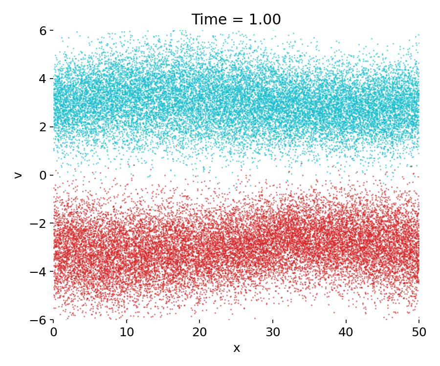
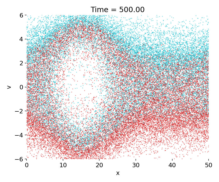
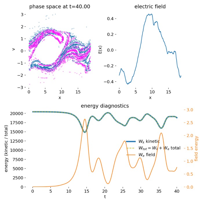
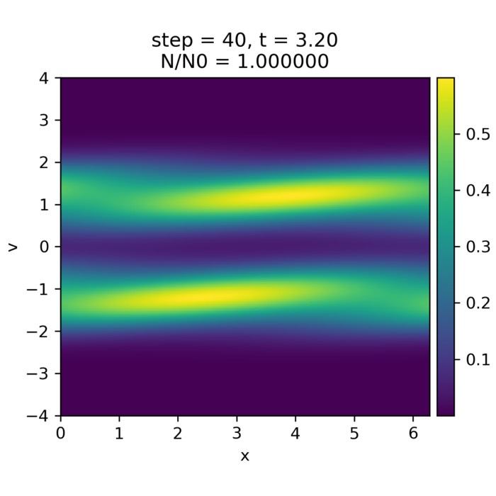
Top to bottom: Phase-space distribution $(x,v)$ of the two-stream PIC simulation at times $t=0$, $t=50$, and $t=499$. At $t=0$, two counter-streaming electron beams are clearly separated in velocity space, with only weak spatial modulation. By $t=50$, the two-stream instability has grown nonlinearly, leading to particle trapping and the formation of coherent phase space vortices. At $t=499$, strong phase-space mixing and filamentation dominate, indicating long-time collisionless evolution after saturation. Red and cyan points denote the two initially counter-streaming beam populations.

At early times, the system is close to the prescribed initial condition: Two counter-streaming electron beams with finite thermal spread and a small sinusoidal velocity perturbation. The phase-space distribution remains approximately homogeneous in position, with only weak correlations between position and velocity. During this stage, the electric field energy is small, and almost all energy resides in particle kinetic energy. The dynamics is dominated by free streaming and the imposed perturbation has not yet grown significantly.

As the simulation progresses, the velocity perturbation seeds the two-stream instability. Around intermediate times, coherent structures begin to emerge in phase space. Particles become trapped in the self-generated electrostatic potential, leading to the formation of characteristic phase space vortices, often referred to as Bernstein–Greene–Kruskal–like structuresꜛ. These vortices mark the nonlinear saturation of the instability: Linear growth gives way to particle trapping, and the system reorganizes its distribution function rather than continuing exponential amplification.

At late times, the phase-space distribution exhibits strong mixing and filamentation. The initially well-separated beams are no longer clearly distinguishable, and fine-scale structures develop as trapped particle populations rotate in phase space. This filamentation is a hallmark of collisionless Vlasov dynamics and reflects the absence of dissipation in the model. While macroscopic quantities may appear quasi-steady, the microscopic phase-space structure continues to evolve.

The energy diagnostics provide a complementary and quantitatively consistent picture. During the early phase, electric field energy grows rapidly at the expense of kinetic energy, reflecting the linear growth of the instability. Once particle trapping sets in, the field energy saturates and oscillates around a characteristic level, while kinetic energy correspondingly decreases and then partially recovers. The total energy remains approximately conserved, as expected for an electrostatic PIC simulation with a symplectic leapfrog particle pusher and periodic boundary conditions.

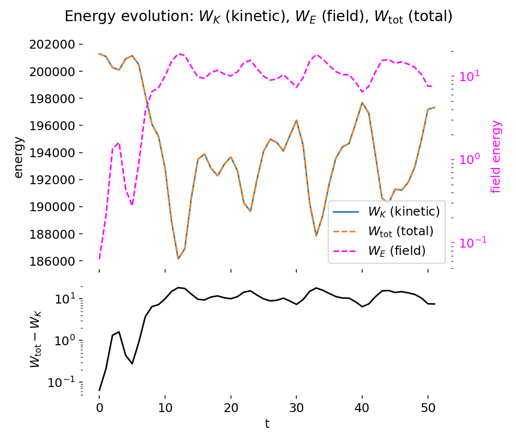
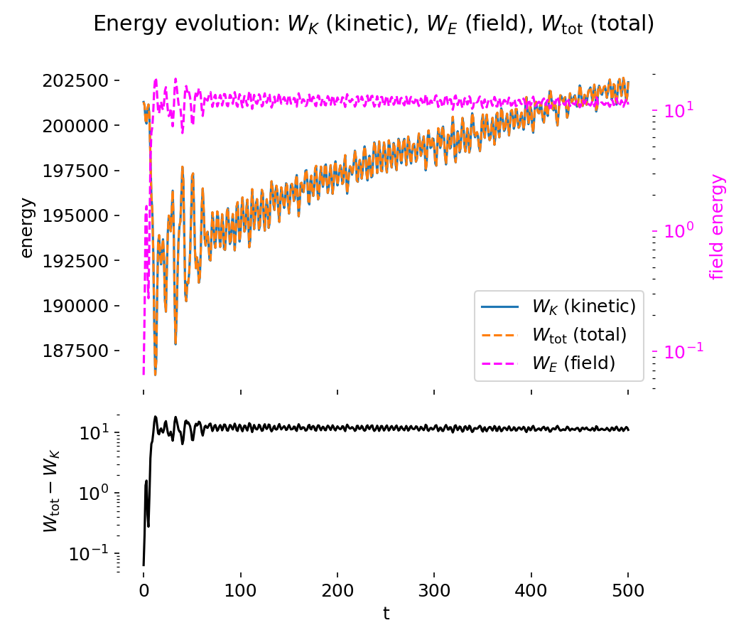
Top to bottom: Energy evolution of the two-stream PIC simulation at $t=50$ and $t=499$. The upper panels show kinetic energy $W_K$, electric field energy $W_E$, and total energy $W_{\mathrm{tot}}$ as functions of time. During the growth phase, electric field energy increases at the expense of kinetic energy, followed by saturation and oscillatory energy exchange due to particle trapping. The lower panels show the difference $W_{\mathrm{tot}} - W_K = W_E$ on a logarithmic scale, highlighting the field energy contribution and confirming approximate total energy conservation over long times.

The difference between total and kinetic energy directly tracks the electric field energy and highlights the reversible energy exchange between particles and fields. Small residual oscillations and slow drifts in total energy are attributable to numerical effects such as finite grid resolution, time-step size, and statistical noise associated with a finite number of macroparticles. Importantly, no secular energy blow-up is observed, indicating stable long-term behavior of the scheme.

Overall, the simulation reproduces the essential physics of the collisionless two-stream instability: Linear growth driven by velocity-space anisotropy, nonlinear saturation via particle trapping, and long-time phase-space mixing. This makes the example a minimal but representative demonstration of how Particle-in-Cell methods capture kinetic plasma phenomena beyond the reach of fluid descriptions, with direct relevance to space and astrophysical plasmas where collisions are negligible.

I thank Philip Moczꜛ for making his code publicly availableꜛ), which served as the basis for this example.

Physical relevance and applications

PIC methods are indispensable wherever kinetic effects dominate plasma behavior. In laboratory plasmas, they are used to study beam–plasma interactions, sheath formation, and wave–particle coupling. In astrophysical and space plasmas, their relevance is even broader.

In space physics, PIC simulations provide insight into collisionless reconnection in the magnetotail, the formation of shocks in the solar wind, and the microphysics of auroral acceleration regions. They allow one to connect in situ spacecraft measurements of particle distributions and fields to underlying kinetic processes. Importantly, PIC simulations often reveal that macroscopic energy conversion proceeds through subtle phase space dynamics rather than through large electromagnetic energy reservoirs.

While PIC methods are computationally expensive and subject to statistical noise, their ability to represent nonthermal distributions and nonlinear wave–particle interactions makes them irreplaceable for many fundamental plasma processes.

Conclusion

The Particle-in-Cell method offers a conceptually clear and physically faithful approach to simulating kinetic plasmas. By combining particle dynamics with grid-based field solvers, it captures collective electromagnetic behavior without sacrificing microscopic detail. Even in its simplest electrostatic form, PIC reveals the essential mechanisms behind plasma instabilities and energy redistribution.

In space physics, PIC simulations serve as a bridge between theory and observation, providing a controlled environment in which kinetic processes can be isolated and understood. As computational resources continue to grow, PIC methods remain a cornerstone of plasma physics, enabling increasingly realistic and detailed explorations of collisionless plasma dynamics.

Update and code availability: This post and its accompanying Python code were originally drafted in 2020 and archived during the migration of this website to Jekyll and Markdown. In January 2026, I substantially revised and extended the code. The updated and cleaned-up implementation is now available in this new GitHub repositoryꜛ. Please feel free to experiment with it and to share any feedback or suggestions for further improvements.

References and further reading

• Wolfgang Baumjohann and Rudolf A. Treumann, Basic Space Plasma Physics, 1997, Imperial College Press, ISBN: 1-86094-079-X
• Treumann, R. A., Baumjohann, W., Advanced Space Plasma Physics, 1997, Imperial College Press, ISBN: 978-1-86094-026-2
• Donald A. Gurnett, Amitava Bhattacharjee, Introduction to plasma physics with space and laboratory applications, 2005, Cambridge University Press, ISBN: 978-7301245491
• Francis F. Chen, Introduction to plasma physics and controlled fusion, 2016, Springer, ISBN: 978-3319223087
• R. C. Davidson, Methods in nonlinear plasma theory, 1972, Academic Press, ISBN: 978-0122054501
• Birdsall, C. K., Langdon, A. B., Plasma Physics via Computer Simulation, 1985/2004, CRC Press, ISBN: 978-0750310253
• Hockney, R. W., Eastwood, J. W., Computer Simulation Using Particles, 1988, CRC Press, ISBN: 978-0852743928
• Dawson, J. M., Particle Simulation of Plasmas, Reviews of Modern Physics, 1983, Rev. Mod. Phys. 55, 403, DOI: 10.1103/RevModPhys.55.403ꜛ
• Nicholson, Introduction to Plasma Theory, 1992, Krieger Publishing Company, ISBN: 978-0894646775
• Blog post “Create Your Own Plasma PIC Simulation (With Python)” on Mediumꜛ (GitHub repositoryꜛ) by Philip Moczꜛ
• Wikipedia article on Bernstein–Greene–Kruskal modesꜛ
• Wikipedia article on Particle-in-Cell methodꜛ