Colocalizing cells
Cell colocalization refers to the spatial overlap or co-occurrence of different cellular components or molecules within a biological sample or an individual cell. It is a measure of the degree to which two or more cellular entities, such as proteins, organelles, or molecules, are present in the same location or region within a cell or tissue. Cell colocalization analysis aims to quantify and characterize the relationship between these entities by examining the extent to which their signals or markers overlap in microscopy images. Technically, the analysis examines the degree of overlap between the distinct fluorescent signals of two or more fluorophores with separate emission wavelengths, which are used to label the cellular components of interest. It can provide valuable insights into cellular processes, interactions between molecules, and functional relationships within cells.
Unfortunately, there is no dedicated plugin for detecting cell colocalization in Napari yet. However, we can bypass this lack by simply performing some “maths” on the segmentation layers of the corresponding cellular components and the enclosing cells, surrounding tissue, or any other region of interest.
 Left: Original image showing cells containing sub-cellular objects (bright spots). Middle: Segmentation of the cells using Cellpose, referred to as the “foreground” $F$ label layer. Right: Segmentation of the sub-cellular objects using StarDist, referred to as the “background” $B$ label layer. Colocalization analysis aims to quantify the degree of overlap between $F$ and $B$. Image source: “test_lsm_ch0” provided in the GitHub data folder (see image credits in the acknowledgements below).
Colocalizing cells in Napari
We refer the segmentation of the cellular components of interest as “foreground” $F$ and the segmentation of the surrounding cell, tissue or any other region of interest as “background” $B$. We are interested in which parts of $F$ overlap (i.e., “colocalize”) with $B$ – if any. This can be achieved by calculating the intersection of $F$ and $B$ and then quantifying the resulting overlap. In principle, the intersection could be calculated by multiplying the corresponding pixel values of the two layers. Since we use the segmentation results obtained, e.g., by global thresholding methods, a Cellpose or StarDist, as described in the previous chapters, our segmented layers $F$ and $B$ are already individually labeled, i.e., the pixel values of both layers are not 1 at all, which would be a prerequisite for pursuing the multiplication approach. We could re-binarize $F$ and $B$, perform the multiplication, and then re-label the resulting layer. However, this would be a rather cumbersome approach. Instead, we split the colocalization problem into two steps and use subtraction rather than multiplication. The following steps guide you through the process:
- Segment the “background” objects, that lay inside the original image or in another channel layer. This steps results into the label layer $B$, containing the segmented “background” labels. You can use one of the segmentation methods described in the previous chapters. These methods work best when the background objects are cells, nuclei or similar. If the background is a tissue or any other broader region of interest, the mentioned methods may have difficulties to segment it, as, for instance, the deep learning based methods are not trained on that. In this case, follow the following approach:
- Create a new shape layer.
- Draw a shape that covers the background region of interest.
- Convert the shape layer to a label layer.
That’s it. With this approach, you can label any arbitrary region of interest. You can also label multiple regions by drawing multiple shapes. - If the shape of background region of interest is rather arbitrary, you can also skip steps 1 to 3 and create the label layer directly. In this case, use the
Paintbrushtool to label the background image parts.
- Segment the “foreground” objects by proceeding as described in step 1. This steps results into the label layer $F$, containing the segmented “foreground” labels.
- Open the Napari Assistant widget plugin via
Tools->Utilities->Assistant. - Now, we perform the following two subtractions:
- First Subtraction: From the Assistant widget, select the
Combine labelsoperation and set in the accordingCombine labelswidget the “foreground” layer $F$ as the first label layer and the “background” layer $B$ as the second label layer (see screenshot below). From the operation dropdown menu, choosebinary_subtract (clesperanto). From this operation, we will get the subtraction $F-B$, i.e., a new layer, that contains all parts of $F$ that lay outside the objects in $B$. The subtraction layer is automatically created by the Assistant and called “Result of binary_subtract…”. You can rename the layer, e.g., to “F-B”, by double-clicking on the layer name in the layer list. - Second Subtraction. Repeat as described for the first subtraction, now choosing the newly generated “F-B”-layer as the second layer of the subtraction operation. This time, the resulting layer will contain all parts of $F$, that lay inside the objects in $B$.
- First Subtraction: From the Assistant widget, select the
 The Assistant widget. Left: First subtraction step: Subtract the “background” segmentation layer $B$ from the “foreground” layer $F$ to get a segmentation mask ($F-B$) for the parts of $F$ non-colocalizing with $B$. Right: Second subtraction step: Subtract the new $F-B$-layer from the “foreground” layer $F$ to get a segmentation mask ($F-(F-B)$) for the parts of $F$ colocalizing with $B$.
The resulting label layer of the first and second subtraction can be used for further analysis, e.g., by applying a measurement operation as described here. Or you can save both layers for any later analysis.
Note: For some reason, you can’t properly close the newly created label layers. The Assistant weirdly reopens them after closing. This is at least the case with my current Napari installation. If you want to perform a colocalization analysis with another image, turn off the visibility of all previous layers and ignore them, or restart Napari. As soon as I notice that this issue has been fixed, I will update this tutorial. If you have any idea how to fix this or notice that I’m missing a crucial step here, please let me know.
 Colocalization analysis example of a 2D single-channel image (here: “47316” from the GitHub data folder, see image credits in the acknowledgements below). The “background” $B$ was manually drawn in a shape layer, while the “foreground” $F$ was segmented with StarDist.
 Colocalization analysis example of a 2D single-channel image (here: “test_lsm_ch0” from the GitHub data folder, see image credits in the acknowledgements below). The “background” $B$ segmented with Cellpose and the “foreground” $F$ with StarDist.
 Colocalization analysis example of a 3D single-channel image (here: “Cells (3D+2Ch)” from the Napari sample dataset). The “background” $B$ segmented with Cellpose and the “foreground” $F$ with StarDist.
Further readings
- Wikipedia article on colocalizationꜛ
- GitHub repository of the Napari Assistant pluginꜛ
- Napari hub page of the napari-assistant pluginꜛ
- Napari hub page of the napari-simpleitk-image-processing pluginꜛ
- GitHub repository of the napari-pyclesperanto-assistant pluginꜛ
Acknowledgements
The data file “test_lsm” used in this tutorial is an excerpt from the example data set of Napari PartSeg pluginꜛ
The data file “47316” used in this tutorial is from the Cell Image Libraryꜛ and has the ID CIL:47316. Please cite as Mark Harding (2014) CIL:47316, Staphylococcus aureus, neutrophil, endothelial cell. CIL. Dataset. doi.org/doi:10.7295/W9CIL47316ꜛ.