Blog
Articles about computational science and data science, neuroscience, and open source solutions. Personal stories are filed under Weekend Stories. Browse all topics here. All posts are CC BY-NC-SA licensed unless otherwise stated. Feel free to share, remix, and adapt the content as long as you give appropriate credit and distribute your contributions under the same license.
tags · RSS · Mastodon · simple view · page 17/20
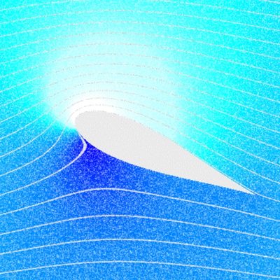
The von Kármán vortex street

One of the most iconic and visually striking examples of unsteady fluid flow is the von Kármán vortex street: The alternating pattern of vortices shed downstream of a bluff body such as a circular cylinder. Beyond its aesthetic appeal, the von Kármán vortex street provides a clean and well-studied setting in which to discuss instability, nonlinear saturation, and the transition from steady to unsteady flow. In this post, we first review the physical and mathematical foundations of vortex shedding and then connect them directly to a concrete numerical implementation based on the lattice–Boltzmann method.
Forced 2D turbulence and Richardson cascade in a pseudospectral vorticity solver

In this post, we implement a forced two dimensional incompressible turbulence simulation in vorticity streamfunction form using a pseudospectral method. We analyze the evolving flow using isotropic energy spectra in wavenumber space to illustrate the Richardson cascade and Kolmogorov type scaling.
Turbulence, Richardson cascade, and spectral scaling in incompressible flows
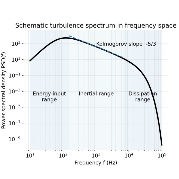
Turbulence is a generic dynamical regime of fluids, independent of whether the medium is liquid, gas, or plasma. In this regime, flow fields become highly complex and appear chaotic. Turbulence is a universal feature of geophysical fluids and largely controls their transport properties, including mixing, momentum transport, and the redistribution of energy across length scales. Despite its ubiquity, turbulence remains one of the central unresolved problems of classical physics, because the governing equations are known, but a closed, predictive theory for the multiscale statistics of turbulent flows is not. A widely used phenomenological picture is the Richardson cascade, which views turbulence as an interacting population of vortices, with energy injected on large scales, transferred by nonlinear interactions across an inertial range, and finally dissipated on sufficiently small scales. In this post, we review the basic concepts of turbulence theory, including the Richardson cascade and Kolmogorov’s phenomenological scaling approach. We also discuss practical aspects of spectral analysis in numerical simulations of forced turbulence.
Hydrodynamics: A brief overview of fluid dynamics and its fundamental equations
Hydrodynamics, the study of fluid motion, is a cornerstone of classical physics with applications ranging from ocean currents to atmospheric circulation. This post provides a brief overview of hydrodynamics, outlining its key concepts, essential properties of fluids, and the fundamental equations that govern fluid behavior: The continuity equation, the Navier–Stokes equation, and the energy equation. We also highlight characteristic features of geophysical fluids and discuss how these principles underpin a wide array of physical phenomena.
A spatially developing 2D Kelvin Helmholtz jet with a finite volume projection method

In this post, we explore the Kelvin-Helmholtz instability in a spatially developing 2D jet using a finite volume projection method on a staggered grid. Building on our previous discussion of the instability in a doubly periodic domain with a pseudospectral method, we now consider a more physically realistic setup with inflow and outflow boundaries. We detail the mathematical formulation, numerical implementation in Python, and present simulation results that highlight the growth and evolution of shear layer perturbations.
Kelvin–Helmholtz instability in 2D incompressible shear flows

The Kelvin–Helmholtz instability is a fundamental fluid dynamical phenomenon that occurs at the interface between two fluid layers moving at different velocities. It plays a crucial role in various natural systems, including atmospheric flows, ocean currents, and space plasmas. In this post, we explore the physical and mathematical description of the Kelvin–Helmholtz instability and present a simple numerical example implemented in Python using a pseudospectral method.
The Lotka-Volterra equations: Modeling predator-prey dynamics
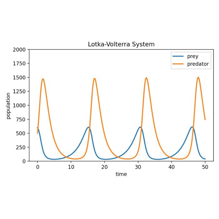
The Lotka-Volterra system, also known as the predator-prey equations, is a mathematical model that describes the interaction between two species: predators and their prey. The system captures the dynamic relationship between the population sizes of predators and prey over time, highlighting the intricate balance between them. In this post we explore this system and calculate its numerical solution using numerical integration Python.
The SIR model: A mathematical approach to epidemic dynamics
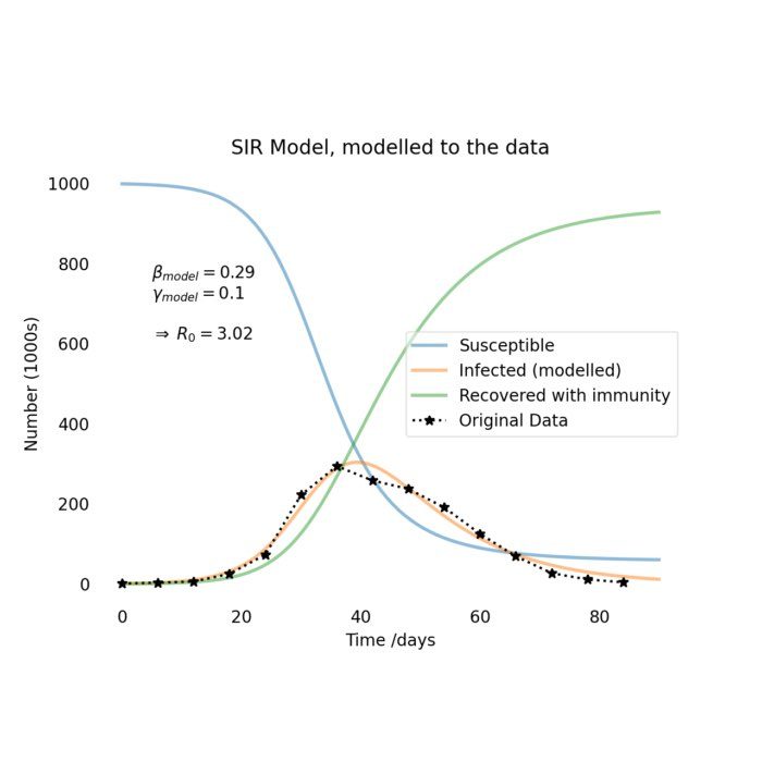
In the wake of the COVID-19 pandemic, epidemiological models have garnered significant attention for their ability to provide insights into the spread and control of infectious diseases. One such model is the SIR model, forming the foundation for studying the dynamics of epidemics. In this blog post, we delve into the details of the SIR model, providing a mathematical description, and showcasing its application through a Python simulation.
Interactive COVID-19 data exploration with Jupyter notebooks
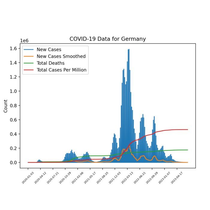
Amidst the ongoing challenges of the COVID-19 pandemic, I have written a Jupyter notebook that facilitates interactive exploration of COVID-19 data. You can select specific countries and visualize key aspects such as confirmed cases, deaths, and vaccinations. The notebook is openly available on GitHub. Feel free to use and share it.
Solving the Lorenz system using Runge-Kutta methods
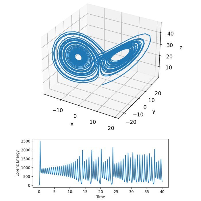
In my previous post, I introduced the Runge-Kutta methods for numerically solving ordinary differential equations (ODEs), that are challenging to solve analytically. In this post, we apply the Runge-Kutta methods to solve the Lorenz system. The Lorenz system is a set of differential equations known for its chaotic behavior and non-linear dynamics. By utilizing the Runge-Kutta methods, we can effectively simulate and analyze the intricate dynamics of this system.