Characteristics of a plasma: Collective behavior, shielding, and intrinsic time scales

June 5, 2020 January 9, 2026 11 minute read see also comments

Most matter encountered in space and astrophysics exists in the plasma state. Roughly 99 percent of the visible matter in the universe is plasma, filling interstellar and intergalactic space, forming stellar interiors and atmospheres, and shaping magnetospheres, solar winds, and accretion flows. On Earth, plasma appears only in limited and often transient contexts, such as lightning, the ionosphere, gas discharges, and laboratory devices. The reason is simple: extended regions of ionized matter are generally hostile to life and require substantial energy input to maintain.

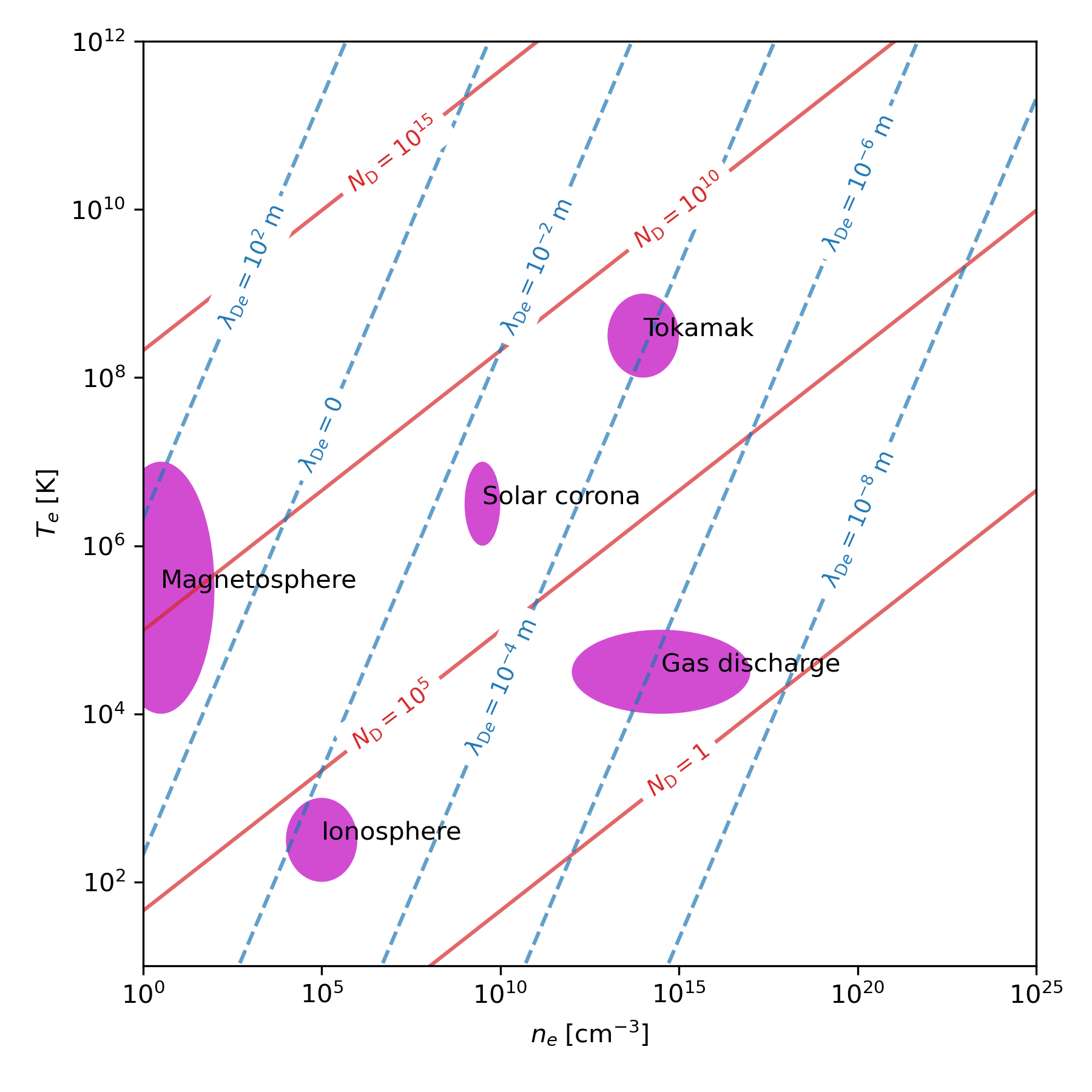
Phase-space overview of plasma regimes in terms of electron density $n_e$ and electron temperature $T_e$. The diagram shows lines of constant Debye length $\lambda_D$ (blue, dashed) and constant number of particles in a Debye sphere $N_D$ (red). Shaded regions indicate typical parameter ranges for different plasma environments, including the magnetosphere, ionosphere, solar corona, gas discharges, and so-called tokamak plasmas. The plot illustrates how plasma classification is governed by collective effects. A system behaves as a plasma only when many particles reside within a Debye sphere ($N_D \gg 1$) and electrostatic interactions are screened on scales larger than $\lambda_D$. The figure is based on code from scipython.comꜛ, used here for illustrative purposes and slightly modified. You can find my modified version of the code on GitHubꜛ.

A plasma is produced when atoms or molecules are ionized, meaning that one or more electrons are removed. The resulting mixture of positively charged ions and free electrons behaves in ways that are qualitatively different from a neutral gas. Importantly, not all plasmas are fully ionized. In so called cold plasmas, only a few percent of the particles carry charge, while the remainder stays neutral. At sufficiently high temperatures, plasmas become fully ionized.

The defining feature of a plasma is not ionization alone, but the emergence of collective electromagnetic behavior. In this post, we introduce the characteristic scales that distinguish a plasma from an ordinary ionized gas and explain how quasineutrality, Debye shielding, and plasma oscillations arise.

A first working definition of a plasma

A plasma can be defined as a quasineutral ensemble of freely moving charged particles that exhibits collective behavior. Quasineutrality means that, on sufficiently large spatial scales, the densities of positive and negative charges are nearly equal. Collective behavior means that particles interact not only through binary collisions, but also through self generated electromagnetic fields that act over long ranges.

Plasma is often referred to as the fourth state of matter, reached by successive energy input that drives matter from solid to liquid, to gas, and finally to an ionized state:

\[\text{Solid} \rightarrow \text{Liquid} \rightarrow \text{Gas} \rightarrow \text{Plasma}.\]

Unlike in a neutral gas, the motion of charged particles in a plasma is intrinsically coupled to electromagnetic fields generated by the plasma itself.

Electromagnetic description and modeling levels

A complete plasma description requires equations for the electromagnetic fields and equations describing the charged matter. Since ions and electrons are treated as free charges, material properties reduce to their vacuum values, and Maxwell’s equations take their simplest form with charge and current densities supplied by the plasma:

\[\begin{align} \nabla \cdot \mathbf{E} &= \frac{\eta}{\epsilon_0}, \\ \nabla \cdot \mathbf{B} &= 0, \\ \nabla \times \mathbf{E} &= -\frac{\partial \mathbf{B}}{\partial t}, \\ \nabla \times \mathbf{B} &= \mu_0 \mathbf{j} + \mu_0 \epsilon_0 \frac{\partial \mathbf{E}}{\partial t}, \end{align}\]

along with equations for matter:

$\begin{align} \mathbf{D} &= \epsilon_0 \mathbf{E}, \\ \mathbf{H} &= \frac{1}{\mu_0} \mathbf{B}\\ \mathbf{j} &= \sigma \mathbf{E}. \end{align}$ where

$\mathbf{E}$ and $\mathbf{B}$ are the electric and magnetic fields,
$\mathbf{D}$ and $\mathbf{H}$ are the electric displacement and magnetic field intensity,
$\eta$ and $\mathbf{j}$ are the charge and current densities,
$\mu_0$ and $\epsilon_0$ are the permeability and permittivity of free space, and
$\sigma$ is the electrical conductivity of the plasma.

Depending on the physical problem, plasmas can be described on different levels:

single particle dynamics
kinetic descriptions using distribution functions
fluid and magnetohydrodynamic models
multifluid and hybrid approaches

Which level is appropriate is determined by the characteristic scales introduced below.

Collective behavior versus neutral gases

In a neutral gas, particles interact primarily through short range collisions. Between collisions, they move independently, and interactions are local and transient.

In a plasma, every charged particle generates electric and magnetic fields that influence many others. Even small charge imbalances produce electric fields that decay only as $1/r$ in vacuum. This long range coupling leads to collective behavior. Local disturbances are communicated through the plasma as a whole, rather than remaining confined to individual particle encounters.

Debye length and the meaning of quasineutrality

Consider a plasma that is quasineutral on average. If a local charge imbalance is introduced, for example by removing some ions from a small region, an electric field develops. Electrons respond to this field and tend to restore neutrality by moving into the depleted region. Whether this response is effective depends on the competition between electrostatic forces and thermal motion.

The characteristic length scale governing this balance is the Debye length,

\[\begin{align} \lambda_D = \sqrt{\frac{\epsilon_0 k_B T_e}{n_e e^2}}, \end{align}\]

where

$T_e$ is the electron temperature
$n_e$ the electron density,
$k_B$ the Boltzmann constant, and
$e$ the elementary charge.

The Debye length measures the distance over which electric potentials are screened by the plasma.

If a charge imbalance extends over a region much smaller than $\lambda_D$, thermal motion dominates and quasineutrality is effectively preserved. If the imbalance extends over distances comparable to or larger than $\lambda_D$, electric fields become significant and the plasma responds collectively.

Quasineutrality therefore holds on spatial scales $L$ that satisfy

\[L \gg \lambda_D.\]

On such scales, the plasma is nearly charge neutral, even though exact equality of ion and electron densities is never achieved.

Debye shielding and charge polarization

Debye shielding provides a concrete illustration of collective plasma behavior. Consider placing a point charge into a plasma. The electric field of this charge attracts oppositely charged particles and repels like charges. As a result, a cloud of opposite charge forms around the test charge, partially canceling its electric field.

Assuming thermal equilibrium and small electrostatic potentials, the resulting electric potential satisfies a screened Poisson equation whose solution is

\[\begin{align} \phi(r) = \frac{q}{4 \pi \epsilon_0} \frac{1}{r} e^{-r/\lambda_D}. \end{align}\]

Compared to the Coulomb potential in vacuum, the field is exponentially suppressed beyond distances of order $\lambda_D$. For $r \ll \lambda_D$, the potential is essentially Coulombic. For $r \gg \lambda_D$, it is strongly attenuated.

This shielding effect depends only on macroscopic plasma parameters such as density and temperature. Individual particle positions do not enter explicitly. The shielding cloud is therefore a collective response of the plasma as a whole.

An illustration of Debye shielding, showing the formation of a Debye sheath around a large positive charge in a plasma. Electrons cluster around the charge, while positive charges shy away from it. This creates a negatively charged cloud, called a sheath, that shields the rest of the plasma from the large positive charge’s influence (i.e. it screens out the large positive charge). The dashed line represents the extent of the cloud, characterized by the Debye length $\lambda_D$ (i.e., $\lambda_D$ is the radius of that sphere). The plot at the bottom shows the electric potential generated by the large positive charge, which falls off as $e^{−r/\lambda_D}/r$ (much steeper than the 1/r one would expect from an unscreened charge). Source: Wikimedia Commons (license: CC0 1.0 public domain).

This qualitative picture of Debye shielding can be made quantitative by examining the electrostatic potential generated by a single test charge embedded in a plasma. In vacuum, the electrostatic potential of a point charge $q$ satisfies Poisson’s equation,

\[\begin{align} \nabla^2 \phi(\mathbf{r}) = - \frac{q}{\epsilon_0} \, \delta(\mathbf{r}), \end{align}\]

with the well-known solution

\[\begin{align} \phi_{\text{vac}}(r) = \frac{q}{4\pi\epsilon_0} \frac{1}{r}, \end{align}\]

which is long-ranged and decays only algebraically with distance.

In a plasma, however, the situation is fundamentally altered. Electrons and ions respond collectively to the electric field of the test charge. Assuming thermal equilibrium and sufficiently small electrostatic potentials, the particle densities can be linearized according to the Boltzmann relation. This leads to the linearized Poisson–Boltzmann equation

\[\begin{align} \nabla^2 \phi(\mathbf{r}) = \frac{1}{\lambda_D^2} \, \phi(\mathbf{r}) - \frac{q}{\epsilon_0} \, \delta(\mathbf{r}), \end{align}\]

where $\lambda_D$ is the Debye length, determined by the plasma density and temperature.

The solution of this equation is the screened Coulomb potential (Yukawa potential),

\[\begin{align} \phi(r) = \frac{q}{4\pi\epsilon_0} \frac{1}{r} \, e^{-r/\lambda_D}. \end{align}\]

For distances $r \ll \lambda_D$, the exponential factor is close to unity and the potential is essentially Coulombic. For $r \gg \lambda_D$, the potential is exponentially suppressed, and the electric field of the test charge becomes negligible.

The following plot illustrates this screening effect by directly comparing the unscreened Coulomb potential with the screened potential for typical plasma parameters. The Debye length emerges as the characteristic distance beyond which electrostatic interactions are effectively short-ranged, demonstrating how collective plasma behavior fundamentally modifies single-particle electric fields.

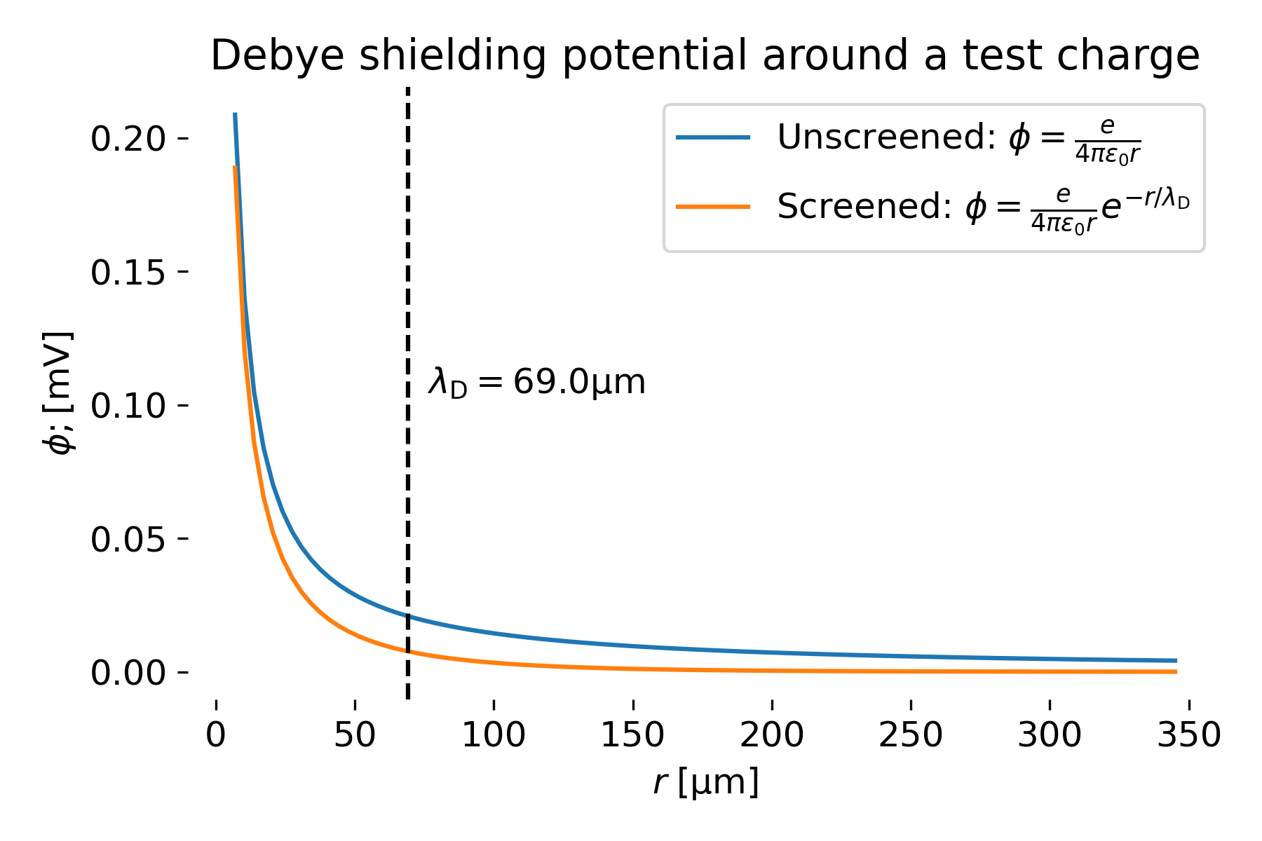
$Electrostatic potential $\phi(r)$ of a test charge embedded in a plasma, illustrating Debye shielding.$
Electrostatic potential $\phi(r)$ of a test charge embedded in a plasma, illustrating Debye shielding. The blue curve shows the unscreened Coulomb potential $\phi \propto 1/r$ expected in vacuum, while the orange curve shows the screened potential $\phi \propto e^{-r/\lambda_D}/r$ arising from collective charge rearrangement in the plasma. The vertical dashed line marks the Debye length $\lambda_D$, which sets the characteristic spatial scale beyond which the electric field of the test charge is exponentially suppressed. Beyond a few Debye lengths, electrostatic interactions between individual charges become negligible, and the plasma remains quasi-neutral. The Python code used to generate this plot is based on scipython.comꜛ’s tutorial “The Debye length”, with modifications. You can find my modified version on GitHubꜛ.

Particle number in the Debye sphere

For Debye shielding to be meaningful, many particles must participate in the shielding process. The number of particles within a sphere of radius $\lambda_D$ is

\[\begin{align} N_D = \frac{4}{3} \pi n \lambda_D^3. \end{align}\]

A necessary condition for plasma behavior is

\[\begin{align} N_D \gg 1. \end{align}\]

If too few particles are present within a Debye sphere, statistical fluctuations dominate and the notion of smooth collective shielding breaks down.

Plasma frequency and intrinsic response times

Quasineutrality is not an instantaneous property of a plasma. If the local balance between electron and ion densities is disturbed, electrons are displaced relative to the ions and experience a restoring electric force. Because ions are much heavier than electrons, they can be treated as stationary on short timescales. The resulting dynamics correspond to collective oscillations of the electron population against an immobile ion background.

To make this explicit, consider a simple one-dimensional model and focus on the electron dynamics. The starting point is the electron continuity equation,

\[\begin{align} \partial_t n_e + \nabla \cdot (n_e v_e) = 0. \end{align}\]

Restricting the problem to one spatial dimension and introducing a small density perturbation around a homogeneous equilibrium,

\[\begin{align*} n_e = n_0 + \delta n_e, \quad \delta n_e \ll n_0, \end{align*}\]

the continuity equation becomes

\[\begin{align} \partial_t n_e + \partial_x \big((n_0 + \delta n_e) v_e \big) = 0. \end{align}\]

Neglecting products of perturbations and linearizing in $\delta n_e$, this reduces to

\[\begin{align} \partial_t \delta n_e + n_0 \, \partial_x v_e = 0. \end{align}\]

The electric field associated with the charge imbalance follows from Gauss’s law,

\[\begin{align} \partial_x E = -\frac{e}{\epsilon_0} \, \delta n_e, \end{align}\]

where the ions are assumed to provide a fixed neutralizing background.

The electron motion is governed by the Lorentz force, which in this electrostatic, one-dimensional setting reduces to

\[\begin{align} m_e \, \partial_t v_e = -e E. \end{align}\]

Combining the linearized continuity equation, Gauss’s law, and the electron equation of motion yields a second-order differential equation for the electron velocity,

\[\begin{align} \partial_t^2 v_e = - \frac{e^2 n_0}{m_e \epsilon_0} \, v_e. \end{align}\]

This is the equation of a harmonic oscillator. Its eigenfrequency is the electron plasma frequency,

\[\begin{align} \omega_{pe} = \sqrt{\frac{e^2 n_0}{m_e \epsilon_0}} \qquad [\mathrm{s}^{-1}], \end{align}\]

which depends only on the electron density and fundamental constants. Expressed as an ordinary frequency,

\[\begin{align} f_{pe} = \frac{\omega_{pe}}{2\pi} \approx 8.16 \, \sqrt{n_e}, \end{align}\]

with $n_e$ measured in $\mathrm{cm}^{-3}$ and $f_{pe}$ in $\mathrm{kHz}$.

The solution corresponds to oscillatory motion of the electrons,

\[\begin{align} v_e(t) \sim e^{\pm i \omega_{pe} t}. \end{align}\]

On timescales shorter than the plasma period

\[\begin{align} T_{pe} = \frac{1}{f_{pe}}, \end{align}\]

charge separation can persist and quasineutrality need not hold. On longer timescales, collective plasma oscillations act to restore it.

The plasma frequency therefore defines the intrinsic response time of a plasma. It is a genuinely collective quantity: the restoring force arises from the self-consistent electric field generated by the displacement of the entire electron population, not from individual particle interactions. This density-dependent timescale plays a central role in distinguishing plasmas from ordinary ionized gases.

Role of neutral particles and collisions

In many environments, plasmas coexist with neutral gas. Collisions between charged and neutral particles tend to suppress collective behavior. If collisions occur more frequently than plasma oscillations, the system behaves more like a neutral gas than a plasma.

A practical condition for plasma behavior is

\[\omega_{pe} \tau_n \gg 1,\]

where $\tau_n$ is the mean time between collisions involving charged particles. Only if the plasma has enough time to respond collectively between collisions do its characteristic properties emerge.

Summary of plasma conditions

A medium can be considered a plasma if the following conditions are satisfied:

The system size is much larger than the Debye length, $L \gg \lambda_D,$ ensuring quasineutrality on macroscopic scales.
Many particles reside within a Debye sphere, allowing collective shielding. $N_D \gg 1.$
The plasma frequency is large compared to collision rates, so that collective dynamics are not suppressed. $\omega_{pe} \tau_n \gg 1.$

Together, these conditions distinguish plasmas from ordinary ionized gases. They establish the physical basis for treating plasmas as media with intrinsic length and time scales and set the stage for more detailed descriptions based on particle dynamics, kinetic theory, or fluid models.

Update and code availability: This post and its accompanying Python code were originally drafted in 2020 and archived during the migration of this website to Jekyll and Markdown. In January 2026, I substantially revised and extended the code. The updated and cleaned-up implementation is now available in this new GitHub repositoryꜛ. Please feel free to experiment with it and to share any feedback or suggestions for further improvements.