A spectral (FFT) Poisson solver for 1D electrostatic PIC
In our previous post on Particle-in-Cell methods, we implemented a minimal 1D electrostatic PIC code using a finite difference Poisson solver. That implementation followed closely the structure of Philip Moczꜛ’s PIC Python codeꜛ. Originally, I had written my own small PIC simulation code, but it did not work at all at that time due to some bugs. After exploring Philip’s code more carefully, however, I went back to my original pure NumPy PIC implementation and fixed the two parts that mattered most: The Poisson solve and the bookkeeping of what exactly is being deposited on the grid. This indeed fixed my code, and I was able to reproduce the two stream instability results shown in the previous post. I thought, it would be useful to share this alternative PIC implementation that uses a spectral Poisson solver based on FFTs, i.e., it differs from the previous post only in how Poisson’s equation is discretized and solved on the grid.
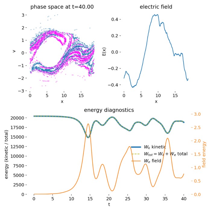
Particle-in-Cell simulation of electron dynamics in a plasma using a spectral Poisson solver via FFTs. The phase space distribution $(x,v)$ of two counter-streaming electron beams is shown at time $t=40.00$. The characteristic vortex-like structures in phase space arise from nonlinear particle trapping in the self-consistent electrostatic potential generated by the two-stream instability. The electric field $E(x)$ exhibits spatial oscillations corresponding to the dominant unstable mode and its harmonics. The simulation captures the essential physics of the collisionless two-stream instability, including linear growth, nonlinear saturation through trapping, and long-time phase space filamentation.
What is different compared to the finite difference variant?
So, what is the difference between the two PIC implementations? Both codes implement the same physical model: A one dimensional, periodic, electrostatic PIC approximation to the Vlasov Poisson system for the two stream instability. The particle advance is conceptually identical in both implementations. The only structural difference is the field solve, meaning how Poisson’s equation is discretized on the grid and inverted to obtain the electric field.
In the electrostatic setting, each macroparticle follows
\[\frac{dx_p}{dt}=v_p,\quad \frac{dv_p}{dt}=\frac{q}{m}E(x_p),\]and the electric field is obtained self consistently from Poisson’s equation. In a periodic domain, it is convenient to write this in potential form,
\[\frac{d^2\phi}{dx^2}=-\rho(x),\quad E(x)=-\frac{d\phi}{dx}.\]A periodic Poisson problem is solvable only if the net charge in the domain is zero. Numerically, this is enforced by removing the $k=0$ Fourier mode, equivalently by subtracting the spatial mean of the deposited source term (for example $\rho\leftarrow\rho-\langle\rho\rangle$ or, in number density form, $n-n_0$ with $\langle n-n_0\rangle=0$). Both implementations apply this neutrality constraint, but they differ in how the remaining modes are inverted.
Finite difference Poisson (grid based linear system)
In the finite difference approach, the second derivative in Poisson’s equation is replaced by a stencil on the grid, yielding a sparse linear system
\[L\,\phi = b,\]where $L$ is the discrete Laplacian and $b$ represents the deposited source term after neutrality enforcement. The electric field is then obtained by applying a discrete gradient operator $G$,
\[E = -G\phi.\]Spectral Poisson solve via FFT (this follow up)
In the FFT based approach used in this post, Poisson’s equation is inverted directly in Fourier space. Writing the deposited source term as $b(x)$, the Fourier coefficients satisfy, for each mode $k\neq 0$,
\[(-k^2)\,\phi_k=b_k \quad\Longrightarrow\quad \phi_k=-\frac{b_k}{k^2},\]and the electric field follows from
\[E_k=-ik\,\phi_k.\]Transforming back with an inverse FFT yields $E(x)$ on the grid, which is then interpolated to particle positions as usual.component to zero.
Key consequences:
- For smooth fields, the spectral inversion is effectively very high order in space. The dominant error is then usually not the Poisson solve itself, but particle noise, deposition and gathering errors, and the time step.
- The cost is $O(N\log N)$ per time step for the field solve, with a small constant factor and no need for linear algebra tuning.
- The method is tied to periodic boundaries and a uniform grid. It is not the right tool if you need sheath boundaries, conductors, or irregular domains.
Practical consequences for accuracy and numerical behavior
So, is there any benefit to using the FFT based Poisson solver instead of the finite difference approach? The answer depends on the specific goals of your simulation. In one dimensional periodic PIC test problems, a spectral Poisson solver offers a particularly clean separation between physics and numerics. Because the inversion of Poisson’s equation is exact for all grid resolved Fourier modes, errors associated with the field solve itself are minimal.
As a result, the numerical behavior of the simulation is dominated by other aspects of the PIC algorithm rather than by the Poisson inversion. In practice, the leading sources of (potential!) numerical error are:
- statistical noise due to the finite number of macroparticles, scaling approximately as $1/\sqrt{N_p}$
- numerical heating caused by inconsistencies between charge deposition and field interpolation
- aliasing of high wave number content if the grid resolution is insufficient to represent emerging phase space structures
- time integration errors if the time step $\Delta t$ is too large compared to characteristic plasma time scales
Numerical implementation
Now that we have discussed the conceptual differences, let’s look at the actual code. The full implementation is given below. It is structured similarly to the finite difference version in the previous post, with the main difference being the poisson_solve_fft_from_n function that implements the spectral Poisson solve via FFTs.
Let’s begin by importing the necessary libraries and setting up some plotting aesthetics:
import os
import numpy as np
import matplotlib.pyplot as plt
import imageio.v2 as imageio

# remove spines right and top for better aesthetics:
plt.rcParams["axes.spines.right"] = False
plt.rcParams["axes.spines.top"] = False
plt.rcParams["axes.spines.left"] = False
plt.rcParams["axes.spines.bottom"] = False
plt.rcParams.update({"font.size": 12})
First, we define the Cloud-In-Cell (CIC) deposition. CIC is a common method for depositing particle properties onto a grid in PIC simulations. It distributes each particle’s contribution to the two nearest grid points based on its position within the cell:
def cic_deposit_number_density(xp, Nx, L):
    """
    CIC number density deposition onto a uniform grid.

    xp : particle positions in [0, L)
    returns:
        n on grid (length Nx), normalized so mean(n) ~ 1
    """
    dx = L / Nx

    g = xp / dx
    i = np.floor(g).astype(int)
    f = g - i

    i0 = i % Nx
    i1 = (i + 1) % Nx

    w0 = 1.0 - f
    w1 = f

    n = np.zeros(Nx, dtype=np.float64)
    np.add.at(n, i0, w0)
    np.add.at(n, i1, w1)

    # convert counts to number density:
    n /= dx

    # normalize so that mean(n) = 1 (for uniform xp distribution).
    # for uniform distribution, expected mean of (counts/dx) is Np/L.
    # multiply by L/Np to get mean ~ 1:
    Np = xp.size
    n *= (L / Np)

    return n
Next, we implement the CIC interpolation to gather the electric field from the grid to the particle positions:
def cic_interpolate_field(Eg, xp, Nx, L):
    """
    CIC interpolation of grid field Eg to particle positions xp.
    """
    dx = L / Nx

    g = xp / dx
    i = np.floor(g).astype(int)
    f = g - i

    i0 = i % Nx
    i1 = (i + 1) % Nx

    w0 = 1.0 - f
    w1 = f

    Ep = Eg[i0] * w0 + Eg[i1] * w1
    return Ep
Here is the spectral Poisson solver using FFTs. This function solves Poisson’s equation in Fourier space and returns the electric field and potential on the grid:
def poisson_solve_fft_from_n(n, n0, L):
    """
    Solve 1D periodic Poisson in normalized form:
        phi'' = -(n - n0)
    then E = -phi'.

    In Fourier space:
        (-k^2) phi_k = (n - n0)_k   =>  phi_k = -(n - n0)_k / k^2  for k != 0

    Returns:
        Eg : electric field on grid (length Nx)
        phi: potential on grid (length Nx)
    """
    Nx = n.size
    dx = L / Nx

    # Fourier wavenumbers (rad / length):
    k = 2.0 * np.pi * np.fft.fftfreq(Nx, d=dx)

    rhs = n - n0
    rhs_k = np.fft.fft(rhs)
    rhs_k[0] = 0.0 + 0.0j  # remove k=0 mode (neutrality)

    phi_k = np.zeros_like(rhs_k)
    mask = (k != 0.0)
    phi_k[mask] = -rhs_k[mask] / (k[mask] ** 2)

    # E_k = - i k phi_k:
    E_k = -1j * k * phi_k

    phi = np.fft.ifft(phi_k).real
    Eg = np.fft.ifft(E_k).real
    return Eg, phi
We need a function to initialize the two stream instability setup, where half the particles have a positive drift and half have a negative drift, with a small perturbation to seed the instability:
def initialize_two_stream(Np, L, vth, v0, seed=0, A=0.05):
    """
    Two drifting Maxwellians:
    * half particles with drift +v0, half with drift -v0, same thermal spread vth
    * positions uniform on [0, L)
    * apply a small sinusoidal velocity perturbation to seed the instability
    """
    rng = np.random.default_rng(seed)
    xp = rng.random(Np) * L

    vp = rng.normal(loc=0.0, scale=vth, size=Np)
    half = Np // 2
    vp[:half] += v0
    vp[half:] -= v0

    # deterministic seed (Mocz-style):
    vp *= (1.0 + A * np.sin(2.0 * np.pi * xp / L))

    return xp, vp
For visualization, we define a helper-function to create a GIF from the (later) saved PNG frames:
def make_gif_from_folder(folder, gif_name, fps=10):
    files = sorted([os.path.join(folder, f) for f in os.listdir(folder) if f.endswith(".png")])
    frames = [imageio.imread(f) for f in files]
    imageio.mimsave(gif_name, frames, fps=fps)
In the main simulation function, we set up the simulation parameters, initialize particles, and run the PIC loop. The electric field is solved using the FFT-based Poisson solver at each time step:
def run_pic_1d_es(
    *,
    Nx=256,
    Np=30000,
    L=2.0 * np.pi,
    dt=0.03,
    nsteps=4000,
    q_over_m=-1.0,
    n0=1.0,
    vth=0.25,
    v0=1.0,
    A=0.05,
    seed=1,
    # output
    results_path="pic_frames_fft_fixed",
    plot_every=200,
    diag_every=10,
    fps=10):
    os.makedirs(results_path, exist_ok=True)

    dx = L / Nx

    # initialize particles:
    xp, vp = initialize_two_stream(Np, L, vth=vth, v0=v0, seed=seed, A=A)

    # initial fields:
    n_grid = cic_deposit_number_density(xp, Nx, L)
    Eg, _ = poisson_solve_fft_from_n(n_grid, n0=n0, L=L)
    Ep = cic_interpolate_field(Eg, xp, Nx, L)

    # leapfrog init: velocities at half step:
    a = q_over_m * Ep
    v_half = vp + a * (0.5 * dt)

    # prepare diagnostics storage:
    t_hist = []
    Wk_hist = []
    We_hist = []
    Wtot_hist = []

    fig = None
    rng_plot = np.random.default_rng(seed + 123)

    for step in range(1, nsteps + 1):
        # drift: x^{n+1} = x^n + v^{n+1/2} dt
        xp = xp + v_half * dt
        xp %= L

        # deposit n(x):
        n_grid = cic_deposit_number_density(xp, Nx, L)

        # field solve:
        Eg, _ = poisson_solve_fft_from_n(n_grid, n0=n0, L=L)

        # gather: E(xp)
        Ep = cic_interpolate_field(Eg, xp, Nx, L)

        # kick: v^{n+3/2} = v^{n+1/2} + (q/m) E dt:
        a = q_over_m * Ep
        v_half = v_half + a * dt

        # diagnostics every diag_every steps:
        if (step % diag_every) == 0:
            # reconstruct v at integer time for diagnostics:
            # v^n = v^{n+1/2} - (q/m) E(x^n) dt/2
            vp_diag = v_half - a * (0.5 * dt)

            # energies (normalized):
            # kinetic: sum 1/2 v^2 (mass=1)
            Wk = 0.5 * np.sum(vp_diag ** 2)

            # field energy: 1/2 ∫ E^2 dx:
            We = 0.5 * np.sum(Eg ** 2) * dx

            t = step * dt
            t_hist.append(t)
            Wk_hist.append(Wk)
            We_hist.append(We)
            Wtot_hist.append(Wk + We)

        # plotting:
        if (step % plot_every) == 0 or step == 1:
            vp_plot = v_half - a * (0.5 * dt)

            if fig is None:
                fig = plt.figure(figsize=(11, 8))
            plt.clf()

            ax1 = plt.subplot2grid((2, 2), (0, 0))
            ax2 = plt.subplot2grid((2, 2), (0, 1))
            ax3 = plt.subplot2grid((2, 2), (1, 0), colspan=2)

            # phase space (subsample):
            n_show = min(6000, Np)
            idx = rng_plot.choice(Np, size=n_show, replace=False)

            # define once, right after initialization (outside the loop):
            beam_id = np.zeros(Np, dtype=int)
            beam_id[:Np//2] = 0
            beam_id[Np//2:] = 1

            # inside plotting, after choosing idx:
            mask0 = beam_id[idx] == 0
            mask1 = ~mask0
            ax1.scatter(xp[idx][mask0], vp_plot[idx][mask0], s=1, alpha=0.5, color="tab:blue")
            ax1.scatter(xp[idx][mask1], vp_plot[idx][mask1], s=1, alpha=0.5, color="magenta")
            ax1.set_xlabel("x")
            ax1.set_ylabel("v")
            ax1.set_title(f"phase space at t={step*dt:.2f}")

            # field E(x):
            xg = np.linspace(0.0, L, Nx, endpoint=False)
            ax2.plot(xg, Eg)
            ax2.set_xlabel("x")
            ax2.set_ylabel("E(x)")
            ax2.set_title("electric field")

            # energy history:
            if len(t_hist) > 2:
                ax3.plot(t_hist, Wk_hist, label="$W_k$ kinetic", c="tab:blue", lw=3.5)
                #ax3.plot(t_hist, We_hist,   label="$W_e$ field", c="tab:green")
                ax3.plot(t_hist, Wtot_hist, '--', label="$W_{tot}=W_k + W_e$ total", c="tab:olive")
                ax3.set_xlabel("t")
                ax3.set_ylabel("energy (kinetic / total)")
                ax3.set_ylim(0, 21000)

                # plot W_e on secondary y-axis:
                ax3r = ax3.twinx()
                ax3r.plot(t_hist, We_hist, label="$W_e$ field", c="tab:orange")
                ax3r.set_ylabel("field energy")
                ax3r.set_ylim(0,3)

                # combined legend:
                lines_l, labels_l = ax3.get_legend_handles_labels()
                lines_r, labels_r = ax3r.get_legend_handles_labels()
                ax3.legend(lines_l + lines_r, labels_l + labels_r, loc="center right", frameon=False)

                # color the right y-axis label to match the line color:
                ax3r.yaxis.label.set_color("tab:orange")
                ax3r.tick_params(axis="y", colors="tab:orange")

                ax3.set_title("energy diagnostics")

            plt.tight_layout()
            plt.savefig(os.path.join(results_path, f"pic_{step:05d}.png"), dpi=150)

    plt.close(fig)

    # GIF
    # for storing the gif, the go the parent folder of results_path:
    print("saving gif...", end="")
    GIF_results_path = os.path.dirname(results_path)
    make_gif_from_folder(results_path, gif_name=os.path.join(GIF_results_path, "pic_evolution.gif"), fps=fps)
    print("done.")

    return {
        "t": np.array(t_hist),
        "Wk": np.array(Wk_hist),
        "We": np.array(We_hist),
        "Wtot": np.array(Wtot_hist),
    }
Finally, we run the simulation with specified parameters. The results, including phase space evolution and energy diagnostics, are saved as PNG frames and compiled into a GIF:
out = run_pic_1d_es(
    Nx=512,             # grid points, e.g., 256; the higher the better resolution but more compute
    Np=40000,           # number of particles
    L=6.0 * np.pi,      # box size
    dt=0.01,            # timestep
    nsteps=80000,       # number of timesteps (simulation time = nsteps*dt)
    q_over_m=-1.0,      # normalized electron charge/mass
    n0=1.0,             # background density
    vth=0.15,           # thermal velocity, e.g., 0.25
    v0=1.0,             # drift velocity of the two streams, e.g., 1.0
    A=0.05,             # amplitude of initial perturbation
    seed=42,            # random seed
    results_path="pic_frames_fft",
    plot_every=200,     # plot every N steps
    diag_every=10,      # diagnostics every N steps
    fps=10,             # frames per second for gif
)
The resulting animation of the two stream instability evolution using the FFT based PIC code. The upper left panel shows the phase space evolution of the two counter streaming electron beams, while the upper right panel displays the electric field. The bottom tracks the kinetic, field, and total energy evolution over time. From the initial linear growth phase to nonlinear saturation and mixing, the simulation captures the key dynamics of the instability.
Discussion of the simulation results
The simulation reproduces the standard nonlinear evolution of the one-dimensional electrostatic two-stream instability governed by the Vlasov–Poisson system. Both the phase space diagnostics and the energy evolution are consistent with the expected sequence of linear growth, nonlinear trapping, and collisionless saturation.
At early times, the system remains close to the prescribed initial condition. Two counter-streaming electron beams are clearly separated in velocity space, and the spatial distribution is nearly homogeneous. The electric field has a small amplitude and is dominated by the imposed sinusoidal seed perturbation together with finite-particle noise inherent to the PIC representation. At this stage, the particle dynamics is essentially ballistic, and almost all energy resides in kinetic form.
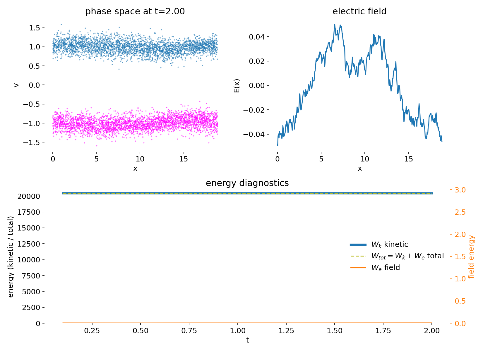
Phase space distribution $(x,v)$ and electric field $E(x)$ shortly after initialization. Two counter-streaming electron beams are clearly separated in velocity space and remain nearly homogeneous in position. The electric field has small amplitude and reflects the imposed sinusoidal seed perturbation together with finite-particle noise. The dynamics is still dominated by free streaming, and no trapping has yet occurred.
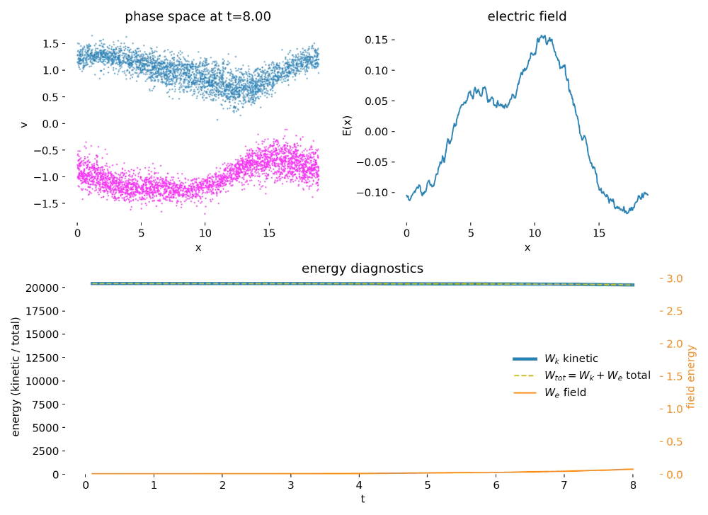
As the instability develops, a resonant electrostatic mode grows due to the velocity-space anisotropy of the distribution function. Once the wave amplitude becomes sufficiently large, particles with velocities close to the phase velocity of the wave become trapped in the self-consistent electrostatic potential. This trapping marks the transition from linear to nonlinear dynamics. In phase space, it manifests as the characteristic roll-up into vortex-like structures associated with closed particle orbits in the wave frame. The apparent overlap of the two initially distinct beam populations reflects phase space transport induced by trapping rather than physical mixing or collisions. Each particle continues to follow Hamiltonian dynamics, and the evolution remains strictly collisionless.
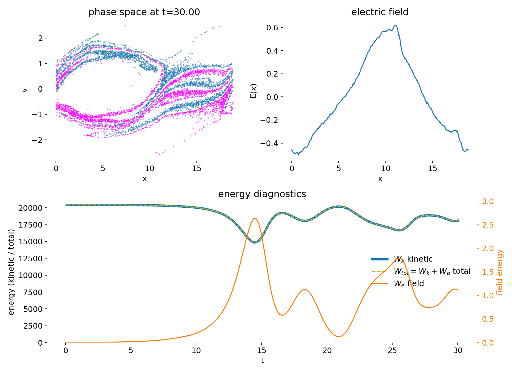
Phase space distribution $(x,v)$ and electric field $E(x)$ during the nonlinear phase. The electrostatic wave has grown to finite amplitude, and particles near the wave phase velocity become trapped in the self-consistent potential. This trapping leads to the formation of characteristic vortex-like structures in phase space. The apparent overlap of the two initially distinct beam populations reflects phase space transport rather than physical mixing.
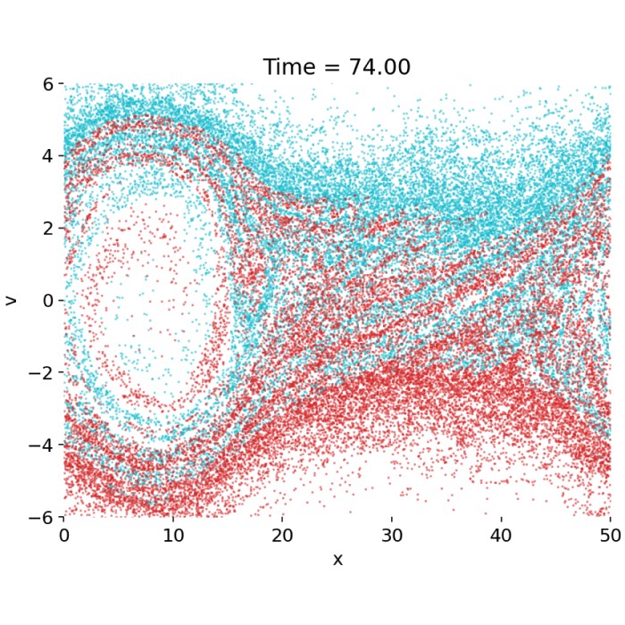
At late times, the instability has saturated. The phase space distribution exhibits strong filamentation and complex fine-scale structure, while the electric field is dominated by long-wavelength modes with superimposed smaller-scale fluctuations. The saturation mechanism is not dissipation but the redistribution of particles in velocity space through trapping, which reduces the free energy available to drive further wave growth. In the absence of collisions, the Vlasov dynamics continues to generate ever finer structures in phase space. In a PIC simulation, this process is ultimately limited by finite particle number, grid resolution, and statistical noise, which act as an effective coarse-graining.
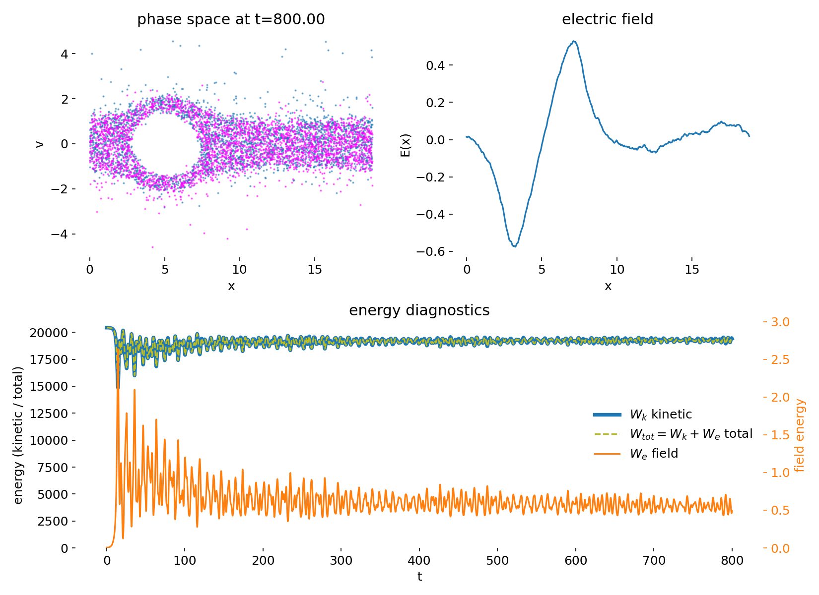
Phase space distribution $(x,v)$ and electric field $E(x)$ at late times after saturation. The instability has redistributed the particle distribution in velocity space, and the phase space structure is dominated by filamentation and fine-scale mixing. The electric field is primarily composed of long-wavelength modes with smaller-scale fluctuations. In the absence of collisions, the Vlasov dynamics continues to generate fine structure, which in PIC is limited by finite particle number and grid resolution.
The energy diagnostics provide a quantitative counterpart to this picture. During the growth phase, electric field energy increases at the expense of particle kinetic energy, reflecting the conversion of directed beam energy into collective electrostatic modes. After saturation, kinetic and field energies oscillate due to reversible energy exchange between particles and the wave. Importantly, the total energy remains approximately conserved throughout the simulation, indicating that the leapfrog particle pusher and the spectral Poisson solver together yield stable long-time behavior without secular energy drift.
Overall, the simulation captures the essential physics of the collisionless two-stream instability: Linear growth driven by velocity-space gradients, nonlinear saturation through particle trapping, and long-time phase space filamentation characteristic of Vlasov dynamics.
Energy conservation comparison to finite difference PIC
Comparing the FFT based simulation presented here to the finite difference based Particle-in-Cell implementation adapted from Philip Mocz, we may notice a qualitative difference in the long time behavior of the energy diagnostics. In the finite difference simulation, the kinetic energy $W_K$ and therefore also the total energy $W_{\mathrm{tot}}$ exhibit a slow but systematic increase over time, whereas in the FFT based simulation the total energy remains approximately constant after the initial transient phase.
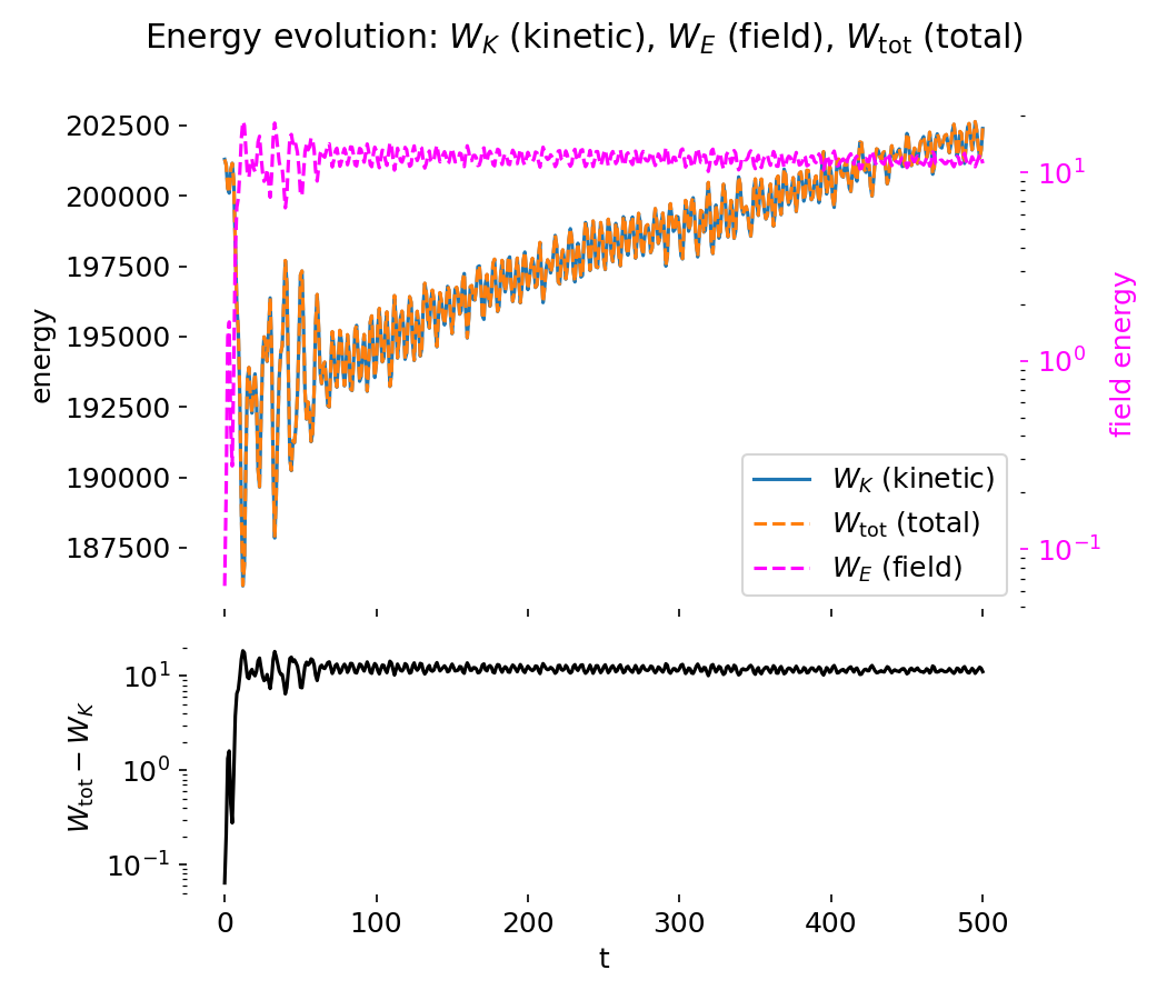
Energy diagnostics of the two-stream PIC simulation using the finite difference based field solver. The upper panel shows the kinetic energy $W_K$, the electric field energy $W_E$, and their sum $W_{\mathrm{tot}}$. The lower panel displays the field energy on a logarithmic scale. A gradual increase of $W_K$ and $W_{\mathrm{tot}}$ is visible over long times.
Both implementations solve the same continuum model, the one-dimensional Vlasov–Poisson system in a periodic domain, and both employ the same conceptual PIC cycle consisting of charge deposition, field solve, field interpolation, and leapfrog particle pushing. The differences in the energy evolution therefore do not reflect different underlying physics, but rather differences in the numerical realization of the field solve and its coupling to the particle dynamics.
In the FFT based implementation, Poisson’s equation is inverted spectrally. After depositing the particle number density $n(x)$ on the grid, the electrostatic potential is obtained in Fourier space via
\[\phi_k = -\frac{(n-n_0)_k}{k^2}, \quad k \neq 0,\]with the zero mode explicitly removed to enforce global charge neutrality. The electric field is then computed as
\[E_k = -\mathrm{i}k\,\phi_k,\]and transformed back to real space. For a fixed grid and periodic boundary conditions, this procedure solves Poisson’s equation exactly up to floating point roundoff. No spatial truncation error is introduced at the level of the field inversion, and the gradient and Laplacian operators are perfectly consistent in spectral space.
As a consequence, after the linear growth and nonlinear saturation of the two-stream instability, the FFT based simulation exhibits a nearly constant total energy. Kinetic and electric field energy are exchanged reversibly through particle trapping and de-trapping, but their sum fluctuates only weakly around a constant mean value. The remaining fluctuations are attributable to finite time step effects, finite particle number noise, and the fact that the discrete PIC system does not exactly preserve all invariants of the continuous Vlasov dynamics. Importantly, however, no systematic secular energy growth is observed.
In the finite difference implementation, Poisson’s equation is solved on the grid using a discrete Laplacian operator, and the electric field is obtained by applying a discrete gradient. While this approach is fully consistent and widely used, it introduces a second order truncation error in space. The discrete Laplacian and gradient are only approximate inverses of one another, and the resulting electric field is therefore not an exact solution of the continuous Poisson problem. Over many time steps, this small inconsistency can accumulate.
In the energy diagnostics, this accumulation appears as a gradual increase of the kinetic energy and, consequently, of the total energy. This behavior should not be interpreted as a physical energy source. Rather, it represents numerical heating, a well known effect in explicit PIC schemes in which small inconsistencies in the field solve and particle push lead to a slow injection of energy into the particle degrees of freedom. The effect becomes particularly visible in long time simulations of collisionless systems, where no physical dissipation is present to damp such errors.
An additional contributing factor is the choice of numerical parameters. In the finite difference setup, the time step is relatively large compared to characteristic plasma time scales, which further amplifies numerical heating in the leapfrog integrator. In contrast, the FFT based simulation employs a significantly smaller time step, reducing time integration errors and improving long term energy behavior independently of the spatial discretization.
The key point is therefore not that one implementation is fundamentally correct and the other incorrect. Both reproduce the same physical mechanism of the two-stream instability, including linear growth, nonlinear saturation through particle trapping, and long time phase space mixing. Rather, the FFT based Poisson solver provides a cleaner separation between physical energy exchange and numerical artifacts in one-dimensional periodic test problems, making it particularly suitable for controlled demonstrations and long time diagnostics.
At the same time, finite difference field solvers generalize naturally to higher dimensions, non periodic geometries, and fully electromagnetic PIC, where FFT based approaches are often impractical. In those settings, careful choice of grid resolution, time step, and particle number is essential to keep numerical heating under control and to ensure reliable long time behavior.
Conclusion
This follow up demonstrated that a minimal electrostatic PIC code can be implemented in two numerically distinct but physically equivalent ways, differing only in how Poisson’s equation is discretized and solved on the grid. By replacing the finite difference Poisson solver with a spectral inversion based on FFTs, the underlying physics of the one dimensional two stream instability remains unchanged, while the numerical properties of the scheme are altered in a transparent and instructive way.
The FFT based implementation reproduces the expected linear growth, nonlinear trapping, and long time phase space filamentation of the Vlasov–Poisson system, while exhibiting markedly improved long time energy behavior in a periodic one dimensional setting. This makes it particularly well suited for pedagogical purposes and for controlled numerical experiments in which energy conservation serves as a sensitive diagnostic of algorithmic consistency.
At the same time, the comparison highlights that numerical heating in PIC simulations is not a failure of the physical model, but a consequence of specific discretization choices, time stepping, and particle field coupling. Finite difference field solvers remain indispensable in higher dimensions and more complex geometries, where spectral methods are no longer applicable, but require correspondingly greater care in parameter selection and diagnostics.
Taken together, the two implementations illustrate a central lesson of kinetic plasma simulation: The physics is encoded in the continuum equations, but the numerical realization strongly shapes how cleanly that physics can be observed in practice.
Update and code availability: This post and its accompanying Python code were originally drafted in 2020 and archived during the migration of this website to Jekyll and Markdown. In January 2026, I substantially revised and extended the code. The updated and cleaned-up implementation is now available in this new GitHub repositoryꜛ. Please feel free to experiment with it and to share any feedback or suggestions for further improvements.
References and further reading
- Wolfgang Baumjohann and Rudolf A. Treumann, Basic Space Plasma Physics, 1997, Imperial College Press, ISBN: 1-86094-079-X
- Treumann, R. A., Baumjohann, W., Advanced Space Plasma Physics, 1997, Imperial College Press, ISBN: 978-1-86094-026-2
- Donald A. Gurnett, Amitava Bhattacharjee, Introduction to plasma physics with space and laboratory applications, 2005, Cambridge University Press, ISBN: 978-7301245491
- Francis F. Chen, Introduction to plasma physics and controlled fusion, 2016, Springer, ISBN: 978-3319223087
- R. C. Davidson, Methods in nonlinear plasma theory, 1972, Academic Press, ISBN: 978-0122054501
- Birdsall, C. K., Langdon, A. B., Plasma Physics via Computer Simulation, 1985/2004, CRC Press, ISBN: 978-0750310253
- Hockney, R. W., Eastwood, J. W., Computer Simulation Using Particles, 1988, CRC Press, ISBN: 978-0852743928
- Dawson, J. M., Particle Simulation of Plasmas, Reviews of Modern Physics, 1983, Rev. Mod. Phys. 55, 403, doi: 10.1103/RevModPhys.55.403ꜛ
- Nicholson, Introduction to Plasma Theory, 1992, Krieger Publishing Company, ISBN: 978-0894646775
- Blog post “Create Your Own Plasma PIC Simulation (With Python)” on Mediumꜛ (GitHub repositoryꜛ) by Philip Moczꜛ
- Wikipedia article on Particle-in-Cell methodꜛ


comments