Neural Dynamics: A definitional perspective
I think it is finally time to define the term “neural dynamics” as I understand it and use it on this blog. The motivation for doing so is both practical and personal. On the practical side, the terms “neural dynamics” and “computational neuroscience” are often used interchangeably, which tends to obscure their respective scope and meaning. On the personal side, I have previously written similar definitional overview posts for other fields, such as space plasma physics and hydrodynamics. These exercises turned out to be useful, primarily because they forced me to make explicit how I mentally structure a field, which topics I consider central, and how different subareas relate to one another. For this reason, it seemed worthwhile to do the same for neural dynamics.
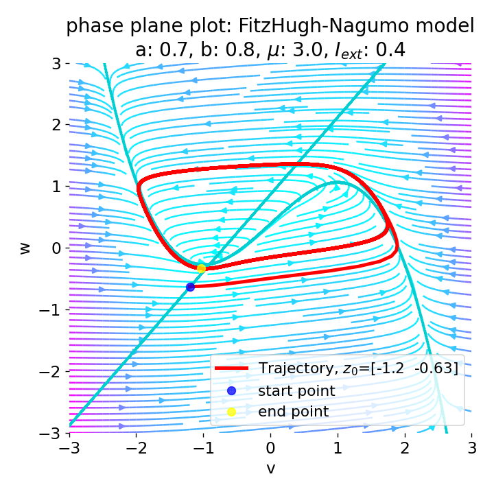
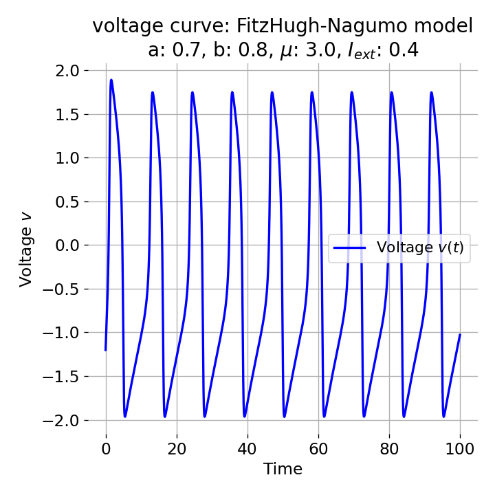
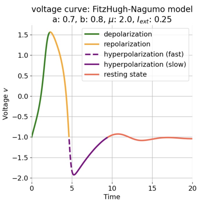
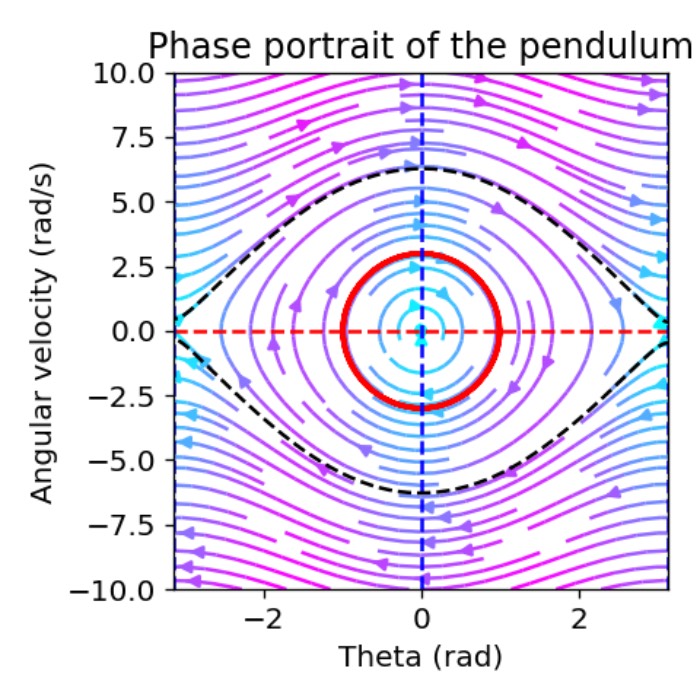
Phase plane (left) and time series (right) of an action potential generated by the FitzHugh–Nagumo model. The left panel shows the nullclines (blue and orange lines) and the trajectory of the system in the phase plane (black line). The right panel shows the membrane potential (voltage) as a function of time, illustrating the rapid rise and fall characteristic of an action potential. Neural dynamics is largely concerned with understanding how such action potentials arise from the underlying biophysical and network dynamics. However, it also goes beyond and studies the dynamics of, e.g., neuronal populations, synaptic plasticity, and learning. In this post, we provide a definitional overview of the field of neural dynamics in order to situate it within the broader context of computational neuroscience and clarify some common misconceptions.
The overview provided in this post is not intended as a textbook chapter, nor as a canonical or exhaustive definition of the field. It is a personal attempt to structure themes, methods, and historical developments in a way that reflects my own focus and trajectory. And: Everything summarized here should be understood as provisional. Both the scientific field and my own understanding of it will continue to evolve, and this overview will almost certainly be extended, refined, or corrected over time. So, if you proceed to read this, please keep in mind that it is a living document rather than a definitive account.
Acknowledgments: My main knowledge of neural dynamics comes from the textbook Neural Dynamicsꜛ by Wulfram Gerstner and colleagues (2014) (among others). I can highly recommend this book to anyone interested in the topic. It provides a comprehensive and mathematically rigorous introduction to the field, covering single neuron dynamics, network models, plasticity mechanisms, and links to cognition. Many of the themes and structures outlined here are inspired by this work.
What is neural dynamics?
Neural dynamics is not identical with computational neuroscience, even though the two are closely related and often confused with each other. Computational neuroscience is best understood as a broad methodological and conceptual framework that uses mathematics, physics, and computational methods to study nervous systems. Within this framework we find a wide range of topics, including biophysical neuron models, network models, learning and plasticity, information coding and decoding, perception and decision making, statistical inference, and data analysis of neural recordings.
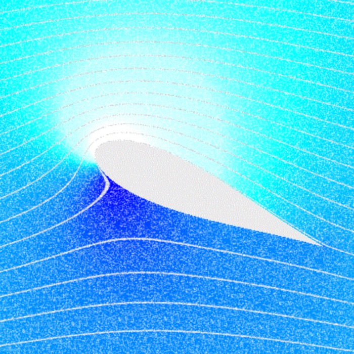
Propagation of an action potential along an axon. An action potential travels along the axon as a spatiotemporal wave of membrane depolarization and repolarization. When the membrane potential reaches threshold, voltage-gated sodium (Na⁺) channels open, leading to rapid depolarization as Na⁺ ions flow into the axon. This is followed by repolarization, driven by the opening of potassium (K⁺) channels and outward K⁺ currents. The resulting change in membrane polarity propagates unidirectionally toward the axon terminal, where it can influence downstream neurons. Neural dynamics studies such processes as dynamical systems, describing how action potentials emerge from underlying biophysical mechanisms, how they propagate in space and time, and how similar principles extend to synaptic interactions, neuronal populations, and network-level activity. Source: Wikimediaꜛ (CC BY-SA 3.0 license)
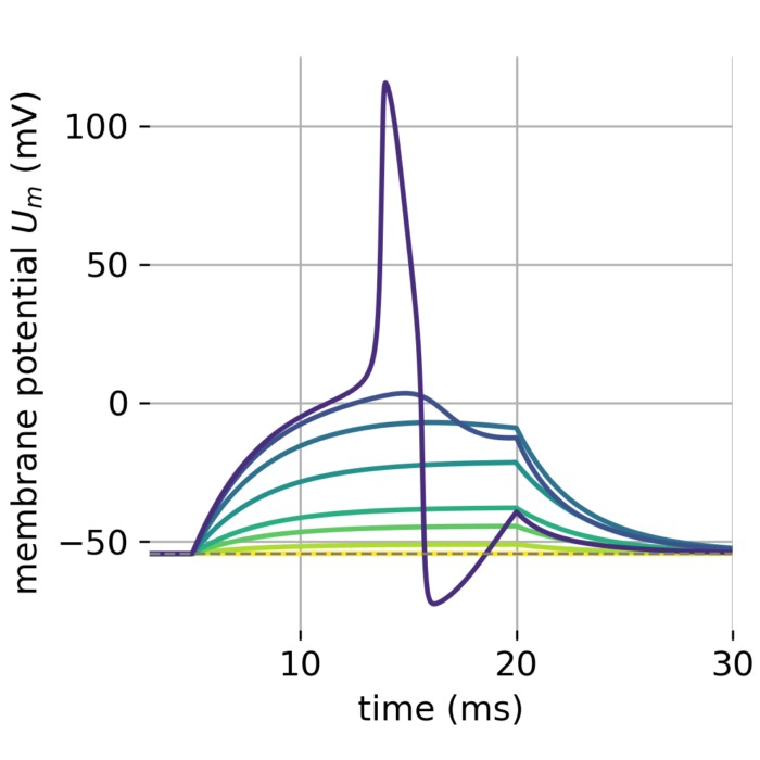
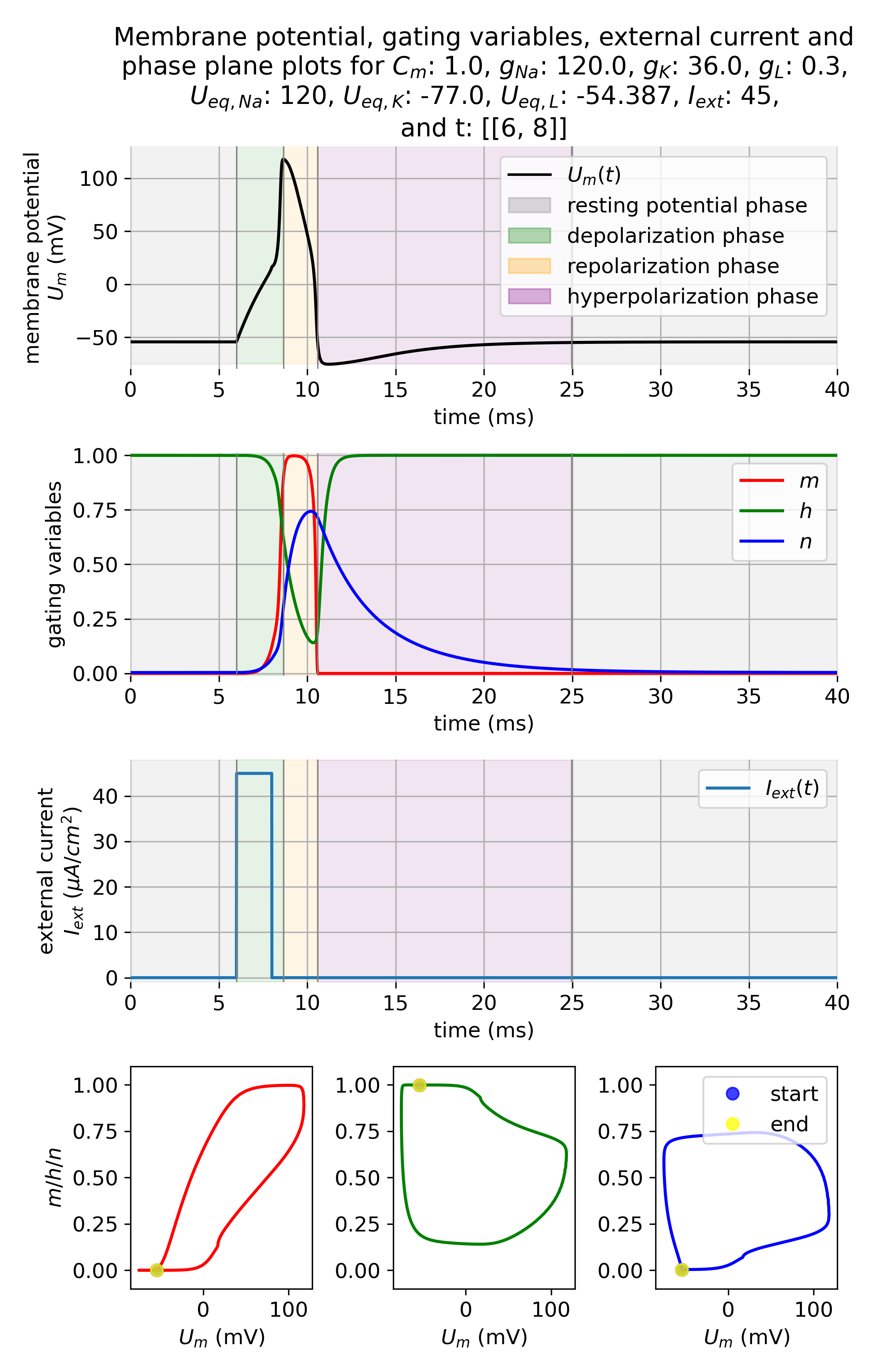 Hodgkin–Huxley dynamics of action potential generation. Shown are the membrane potential $U_m(t)$, the gating variables $m$, $h$, and $n$, the external input current $I_{\mathrm{ext}}(t)$, and corresponding phase-plane projections during the generation of an action potential. A brief but strong external current pulse ($I_{\mathrm{ext}} = 45\,\mu\mathrm{A/cm}^2$ applied for 3 ms) drives the system across threshold, triggering a rapid excursion in state space that corresponds to spike initiation. The subsequent evolution is governed by the coupled nonlinear dynamics of sodium and potassium channel gating, leading to repolarization and afterhyperpolarization. In neural dynamics, the Hodgkin–Huxley model serves as a canonical example of how discrete events such as spikes emerge from continuous-time nonlinear dynamical systems, and how neuronal excitability can be understood geometrically in terms of trajectories, thresholds, and phase-space structure.
Neural dynamics refers more specifically to the study of time dependent neural activity and the mathematical structures that govern it. The focus lies on how neural states evolve in time, how stable or unstable activity patterns arise, how transitions between regimes occur, and how learning reshapes these dynamics. Typical objects of study include membrane potentials, spike trains, synaptic variables, population activity, and low dimensional representations thereof.
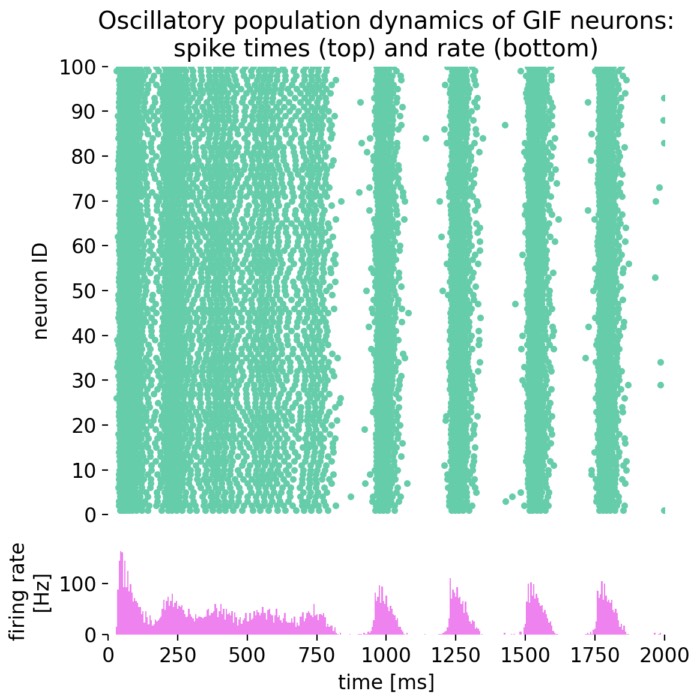
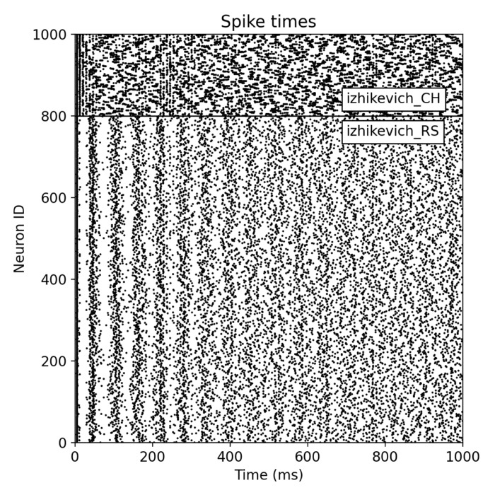
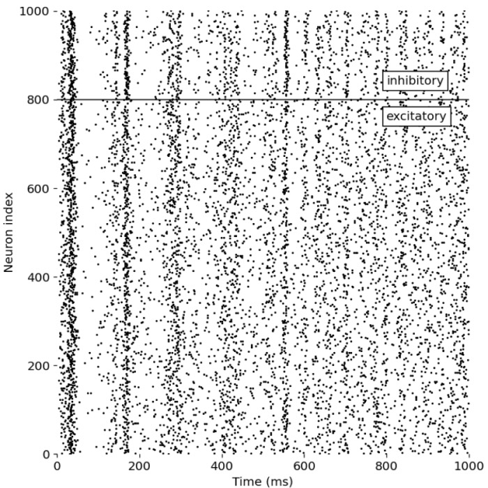
_Ni_low-threshold spiking (LTS).png) Spiking activity in a recurrent network of model neurons (Izhikevich model). Shown are the spike times of all neurons in a recurrent spiking neural network as a function of time. The network consists of 800 excitatory neurons with regular spiking (RS) dynamics and 200 inhibitory neurons with low-threshold spiking (LTS) dynamics, separated by the horizontal line. Each vertical mark corresponds to an action potential (spike) emitted by a single neuron. In the context of neural dynamics, this representation illustrates how single-neuron events, such as the action potentials described above, combine to form structured, time-dependent activity patterns at the network level. Such spiking rasters provide a direct link between microscopic neuronal dynamics and emerging population activity, which can later be analyzed in terms of collective states, low-dimensional structure, and neural manifolds.
Spiking activity in a recurrent network of model neurons (Izhikevich model). Shown are the spike times of all neurons in a recurrent spiking neural network as a function of time. The network consists of 800 excitatory neurons with regular spiking (RS) dynamics and 200 inhibitory neurons with low-threshold spiking (LTS) dynamics, separated by the horizontal line. Each vertical mark corresponds to an action potential (spike) emitted by a single neuron. In the context of neural dynamics, this representation illustrates how single-neuron events, such as the action potentials described above, combine to form structured, time-dependent activity patterns at the network level. Such spiking rasters provide a direct link between microscopic neuronal dynamics and emerging population activity, which can later be analyzed in terms of collective states, low-dimensional structure, and neural manifolds.
In this sense, neural dynamics forms a central but not exhaustive subfield of computational neuroscience. It provides the dynamical backbone on which many other questions rest, but it does not by itself encompass the full scope of computational approaches to brain function. Topics such as Bayesian decoding, normative theories of perception, or purely statistical models of neural data may rely on dynamical assumptions, yet are not primarily concerned with the dynamical systems themselves.
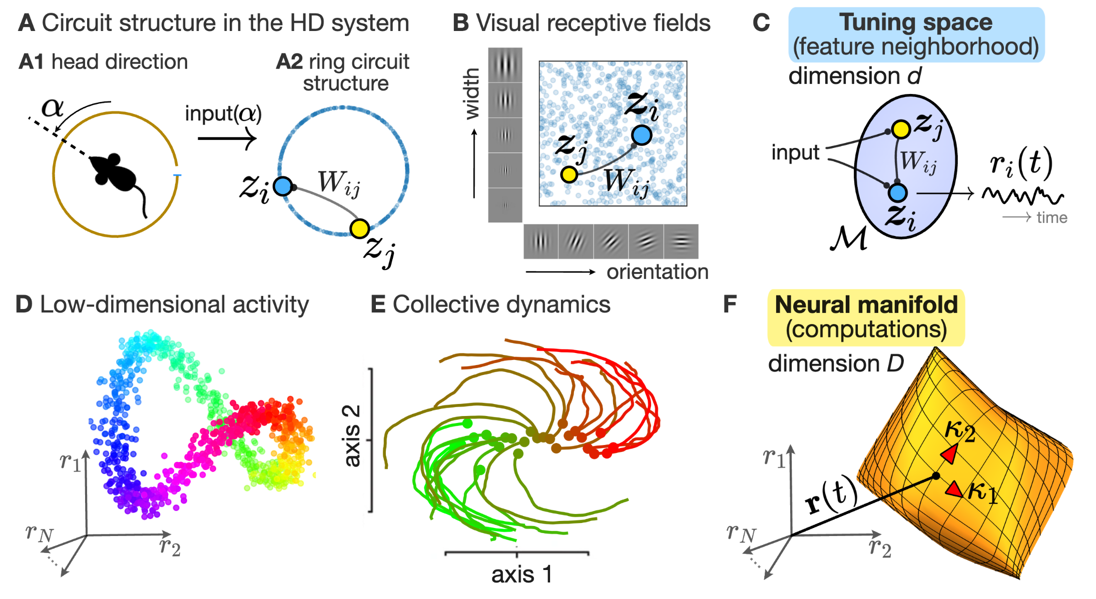 Two complementary perspectives on population activity in neural dynamics. The figure contrasts a “circuit” perspective with a “neural manifold” perspective. In circuit models, neurons are organized in an abstract tuning space, where proximity reflects tuning similarity, and recurrent connectivity $W_{ij}$ together with external inputs generates time-dependent firing rates $r_i(t)$ (panels A–C). In the neural manifold view, the joint activity vector $r(t)\in\mathbb{R}^N$ of a recorded population evolves along low-dimensional trajectories embedded in a high-dimensional space (panels D–F). This is illustrated by ring-like manifolds for head-direction representations and by rotational trajectories in motor cortex, both of which can often be captured by a small number of latent variables $\kappa_1(t),\ldots,\kappa_D(t)$ with $D\ll N$. In the context of our overview post here, I think, the figure highlights very well why neural dynamics naturally connects mechanistic network modeling with state-space descriptions of population activity. These are not competing accounts, but complementary levels of description that emphasize different aspects of the same underlying dynamical system. Source: Figure 1 from Pezon, Schmutz, Gerstner, Linking neural manifolds to circuit structure in recurrent networks, 2024, bioRxiv 2024.02.28.582565, doi: 10.1101/2024.02.28.582565ꜛ (license: CC-BY-NC-ND 4.0)
The focus I adopt here is explicitly on neural dynamics as it appears in spiking neuron models, recurrent networks, and plasticity driven systems. Integrate and fire models, conductance based neurons, spiking neural networks, and learning rules such as spike timing dependent plasticity fall squarely into this domain. This decision reflects a weighting rather than an exclusion. It simply marks the region of computational neuroscience where dynamical systems theory and time continuous modeling play the most prominent role.
In short:
Computational neuroscience is the broad field that uses computational methods to study the brain, while neural dynamics is the subfield that focuses on the time dependent evolution of neural activity and the mathematical structures that govern it.
A mathematical backbone for neural dynamics
What I have learned so far is that, unlike classical [hydrodynamics]/blog/2021-03-04-hydrodynamics/ or magnetohydrodynamics, neural dynamics does not possess a single, closed set of governing equations from which all models can be derived. The diversity of biological mechanisms and levels of description precludes such a unifying formulation. Nevertheless, there exists a common mathematical backbone that underlies most models used in neural dynamics.
At its core, neural dynamics studies systems of coupled, nonlinear, and often stochastic differential equations. A generic formulation can be written as
\[\begin{align} \frac{d\mathbf{x}}{dt} = \mathbf{F}(\mathbf{x}, \mathbf{I}(t), \boldsymbol{\theta}) + \boldsymbol{\eta}(t). \end{align}\]Here, $\mathbf{x}(t)$ denotes the state vector of the system. Depending on the level of description, this vector may contain membrane potentials, gating variables, synaptic conductances, adaptation currents, or abstract firing rate variables. The function $\mathbf{F}$ encodes the deterministic dynamics, including intrinsic neuronal properties, synaptic coupling, and nonlinear interactions. External inputs are represented by $\mathbf{I}(t)$, model parameters by $\boldsymbol{\theta}$, and $\boldsymbol{\eta}(t)$ denotes stochastic terms capturing intrinsic noise or unresolved microscopic processes.
Specific neuron models correspond to particular choices of $\mathbf{F}$. For example, conductance based models yield systems of nonlinear ordinary differential equations with biophysically interpretable parameters. Integrate and fire models reduce this structure to a lower dimensional system with a threshold and reset condition, effectively introducing hybrid dynamics that combine continuous evolution with discrete events. Network models arise when many such units are coupled through synaptic variables that themselves obey additional dynamical equations.
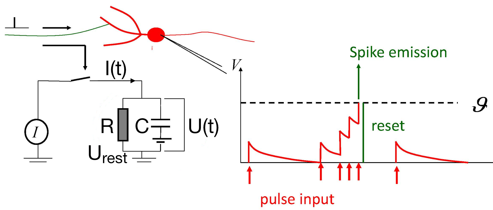
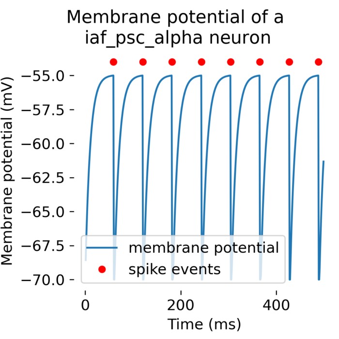
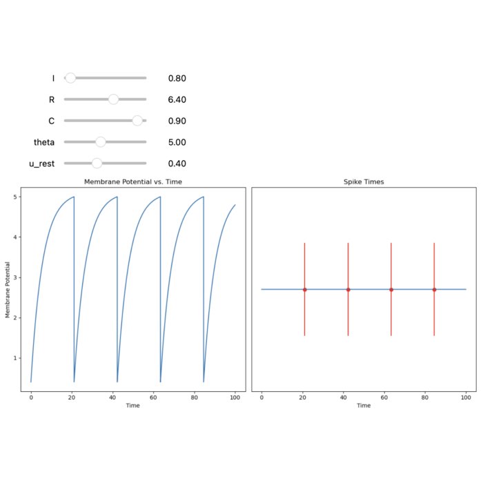
Left: RC equivalent circuit of an Integrate-and-Fire model neuron. The “neuron” in this model is represented by the capacitor $C$ and the resistor $R$. The membrane potential $U(t)$ is the voltage across the capacitor $C$. The input current $I(t)$ is split into a resistive current $I_R$ and a capacitive current $I_C$ (not shown here). The resistive current is proportional to the voltage difference across the resistor $R$. The capacitive current is proportional to the rate of change of voltage across the capacitor. $U_\text{rest}$ is the resting potential of the neuron, which is the membrane potential when the neuron is not receiving any input. Right: The response $U(t)$ on current pulse inputs. When the neuron receives an input current, the membrane voltage changes. The Integrate-and-Fire model describes how the neuron integrates these incoming signals over time and fires an action potential once the membrane voltage exceeds a certain threshold (here depicted as $\vartheta$). Modified from this source: Wikimediaꜛ (CC BY-SA 4.0 license)
Plasticity introduces a further layer of dynamics. Synaptic weights become time dependent variables, often governed by equations of the form
\[\begin{align} \frac{dw_{ij}}{dt} = G(x_i, x_j, t), \end{align}\]where $w_{ij}$ denotes the synaptic efficacy from neuron $j$ to neuron $i$, and $G$ implements a learning rule such as spike timing dependent plasticity or a more general three factor rule. The full system then becomes a coupled dynamical system on multiple time scales, with fast neuronal dynamics and slower synaptic adaptation.
From this perspective, neural dynamics is fundamentally the study of high dimensional nonlinear dynamical systems, their fixed points, limit cycles, attractors, bifurcations, and transient trajectories, as well as the ways in which learning reshapes the underlying phase space.
Thematic overview
In this section, I try to maintain a thematic map of neural dynamics as far as I discover the field. Especially this section is likely to evolve over time as I read more and refine my understanding. Therefore, please consider this as a provisional outline rather than a definitive structure.
The map is largely inspired by the organization of Wulfram Gerstner’s Neuronal Dynamics (2014). It closely follows the conceptual progression of that book, while extending it in places to reflect later developments and my own focus. Also note: All topics listed below are understood as interconnected aspects of neural dynamics rather than as isolated modules.
Neurons and biophysical foundations
- The Hodgkin–Huxley model of action potential generation
- Phase plane analysis as a tool for understanding dynamical systems
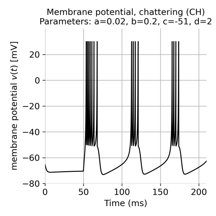
- Reduced neuron models: FitzHugh–Nagumo, Morris–Lecar, Izhikevich models
- Spike initiation dynamics and threshold phenomena
- Synaptic dynamics: Conductance based and current based synapses
- Dendritic processing and compartmental models
Integrate-and-fire neuron models
- The Leaky integrate-and-fire (LIF) model
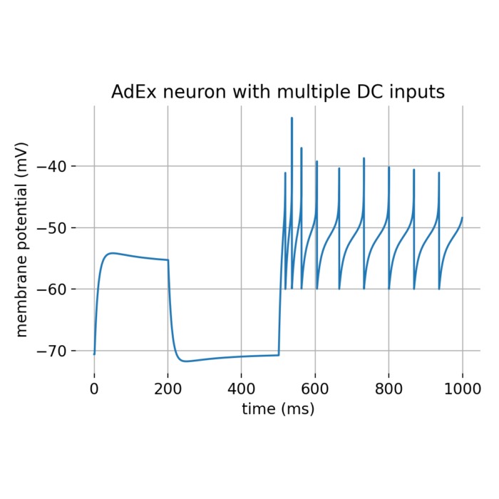
- Exponential integrate-and-fire (EIF) and adaptive exponential integrate-and-fire (AdEx) models
- Generalized integrate-and-fire neuron models
- Nonlinear integrate-and-fire models
- Noisy input and output models
Neuronal populations and network dynamics
- Neuronal populations
- Tuning curves and population coding
- Continuity equation and the Fokker–Planck approach
- Quasi-renewal theory and integral equation approaches
- Fast transients and rate models
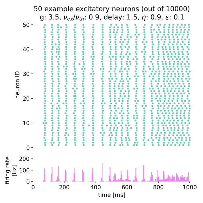
- Asynchronous irregular states in spiking networks (Brunel network)
- Neural state space and latent space representations
Cognitive and systems-level dynamics
- Memory and attractor dynamics
- Cortical field models for perception
- Latest developments in dynamical theories of cognition (incomplete):
- Representational drift in hippocampus and cortex
Synaptic plasticity and learning
- Synaptic plasticity and learning rules
- Three-factor learning rules
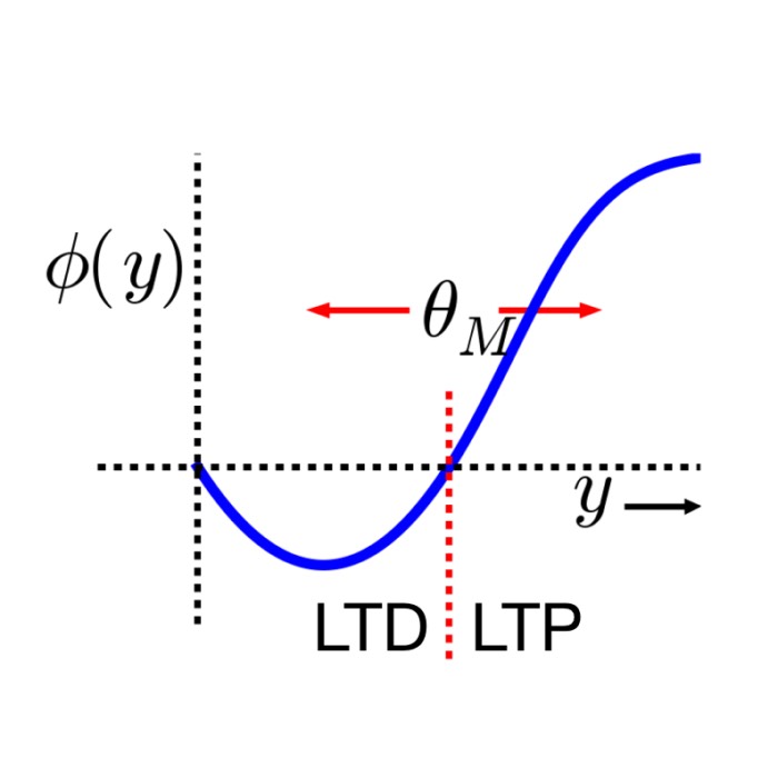
- Bienenstock–Cooper–Munro (BCM) rule
- Voltage-based plasticity rules (e.g. Clopath rule)
- Synaptic tagging and capture (STC)
- Spike-timing-dependent plasticity (STDP)
- In this post, we apply STDP to a pattern recognition task as an example of how it can be used for learning in spiking neural networks.
- Behavioral time-scale synaptic plasticity (BTSP)
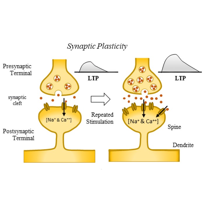
- Long-term potentiation (LTP) and long-term depression (LTD)
- Dendritic prediction and credit assignment (Urbanczik–Senn plasticity)
Dynamical (and stochastic) phenomena in neural systems
- Stability and instability of neural activity patterns
- Transitions between dynamical regimes and state changes
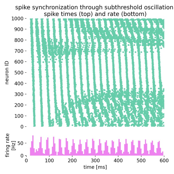
- Oscillatory activity and synchronization phenomena
- Phase oscillator models and synchronization (Kuramoto model)
- Irregular and chaotic dynamics in recurrent neural systems
- Noise-driven variability and stochastic effects in neural activity
Neural dynamics and signal processing
- Backpropagation through time (BPTT)
- Backpropagating action potentials (bAPs)
- Calcium dynamics and calcium waves
From biological to artificial networks and machine learning
- Eligibility traces and Eligibility propagation (e-prop)
- Trainable spiking neural networks for computation and learning
- Energy-based and variational formulations of neural dynamics
Historical overview
Neural dynamics and computational neuroscience did not emerge fully formed, but developed gradually through contributions from physiology, physics, mathematics, and computer science. The following table highlights selected milestones that are particularly relevant for the dynamical perspective.
| Year | Development | Significance | |
|---|---|---|---|
| 1891 | 🧠 | Santiago Ramón y Cajal formulates the neuron doctrine | Establishes neurons as discrete anatomical and functional units of the nervous system |
| 1907 | 📝 | Lapicque introduces the integrate and fire abstraction | Early reduction of excitability to leaky integration with threshold, a prototype for later point neuron models |
| 1909 | 📝 | Campbell’s theorem for shot noise | Mathematical foundation for relating stochastic spike trains to mean rates and variances |
| 1926 | 🔬 | First extracellular recordings of action potentials (Adrian & Zotterman) | Demonstrates that spikes can be recorded extracellularly and linked to sensory stimulation |
| 1931 | 📝/🔬 | Maria Goeppert-Mayer predicts two-photon absorption | Theoretical foundation of nonlinear optical excitation, later enabling two-photon laser scanning microscopy |
| 1943 | 📝 | McCulloch and Pitts formalize threshold units as logical elements | First widely cited mathematical idealization of neurons as binary threshold devices, linking networks to computation |
| 1949 | 🔬 | First intracellular recordings with sharp electrodes (Ling & Gerard) | Enables direct measurement of membrane potentials in single neurons |
| 1949 | 📝 | Hebb formulates cell assemblies and the Hebbian learning principle | Puts synaptic modification and association at the center of learning theory, motivating later plasticity rules |
| 1951 | 🧠/🔬 | Eccles et al. describe local field potentials (LFP) in cerebral cortex | Establishes mesoscopic population signals reflecting synaptic and network activity |
| 1951 | 📝 | Siegert approximation for first passage times | Enables analytical estimation of firing rates for threshold driven stochastic processes |
| 1952 | 📝 | Hodgkin and Huxley conductance based membrane model | Establishes mechanistic ODEs for spikes via voltage dependent gating, defining modern single neuron dynamics |
| 1957 | 📝 | Rall emphasizes dendritic cable properties and compartmental thinking | Provides the foundation for spatially extended neuron models and dendritic integration as a dynamical process |
| 1958 | 📝 | Rosenblatt’s perceptron | Early trainable neural network model, historically important for learning rules and the connectionist line of thought |
| 1961 | 📝 | FitzHugh reduction of Hodgkin and Huxley | Introduces a planar excitable system, enabling phase plane analysis of spikes, nullclines, and excitability types |
| 1962 | 📝 | Nagumo and colleagues’ circuit implementation of excitable dynamics | Concrete electronic realization of excitable systems, helping to popularize reduced excitable models |
| 1963 | 🏅 | Nobel Prize in Physiology or Medicine (Hodgkin & Huxley, shared with Eccles) | Honors the quantitative, biophysical theory of action potential generation that laid the foundation for modern neural dynamics |
| 1965 | 📝 | Stein’s leaky integrate and fire neuron with noise | Establishes stochastic LIF as a canonical rate generating model |
| 1970ies | 📝 | Rate based neuron models (early formalizations) | Introduces continuous firing rate dynamics as an alternative to explicit spikes; first models by Wilson and Cowan (1972–1973) |
| 1970ies | 🔬 | Neher & Sakmann develop the patch clamp technique | Revolutionizes single neuron electrophysiology by enabling high resolution recordings of ionic currents |
| 1971 | 📝 | Ricciardi formulation of diffusion approximations | Formal mathematical framework for firing rate statistics in noisy neurons |
| 1971 | 🧠 | Discovery of place cells in the hippocampus (O’Keefe & Dostrovsky) | Demonstrates location-specific firing of single neurons, establishing a neural basis for spatial representation |
| 1972 | 📝 | Wilson and Cowan population activity equations | Canonical mean field style dynamics for interacting excitatory and inhibitory populations, a workhorse for cortex scale dynamics |
| 1975 | 📝 | Kuramoto phase oscillator model | Canonical model for synchronization and collective dynamics in coupled oscillator systems, later applied to neural rhythms |
| 1975/1977 | 📝 | Amari neural field equations | Spatially continuous rate dynamics and pattern formation in cortex scale models |
| 1978 | 🔬 | Voltage-sensitive dye imaging used to potentially measure action potentials by Cohen & Salzberg | Voltage-sensitive dyes enable optical recording of fast membrane potential changes across neural populations |
| 1982 | 📝 | Hopfield networks as dynamical associative memory | Makes attractor dynamics central for memory and computation, with an explicit energy like Lyapunov function framework |
| 1982 | 📝 | Bienenstock, Cooper, Munro (BCM) synaptic modification theory | Establishes a sliding threshold plasticity principle, influential as a stability mechanism and a bridge between activity statistics and learning |
| 1984 | 🧠 | Discovery of head direction cells (Ranck) | Identifies neurons encoding the animal’s directional heading, introducing orientation as a dynamical neural variable |
| 1986 | 📝 | Rumelhart, Hinton, Williams backpropagation | Not biologically plausible, but historically central for learning in neural networks |
| 1988 | 📝 | Sompolinsky, Crisanti, Sommers chaos in random recurrent networks | Introduces a mathematically controlled route to chaos in high dimensional neural dynamics via random connectivity |
| 1990 | 🔬 | Two-photon laser scanning microscopy (Denk, Strickler & Webb) | Allows deep-tissue optical imaging with cellular resolution in scattering brain tissue |
| 1991 | 🏅 | Neher & Sakmann receive Nobel Prize for patch clamp technique | Enables high resolution recordings of ionic currents and membrane potentials, revolutionizing single neuron physiology |
| 1996 | 📝 | van Vreeswijk and Sompolinsky balanced excitation and inhibition in cortical circuits | Formalizes the balanced state idea as a mechanism for irregular activity and fast responses in large networks |
| 1997 | 🔬 | First genetically encoded calcium indicators (GECIs; here: Cameleon) by Miyawaki et al. | Opens the door to long-term optical recording of neural population activity |
| 1997 | 🔬 | First genetically encoded voltage indicators (GEVIs; here. Flash) by Siegel & Isacoff | Establishes genetically targetable optical reporters of membrane potential dynamics |
| 1997 | 📝 | Spiking neurons as computational units (Maass) | Formal proof that networks of spiking neurons constitute a distinct and powerful computational model |
| 1998 | 📝 | van Vreeswijk and Sompolinsky chaotic balanced state (extended analysis) | Detailed theory of balanced networks, linking microscopic chaos to stable macroscopic activity statistics |
| 1998 | 📝 | Bi and Poo spike timing dependent synaptic modification | Establishes experimentally grounded timing windows for plasticity, pushing “Hebb” into a temporally precise rule |
| 2000 | 📝 | Brunel dynamics of sparsely connected E I spiking networks | Unifies asynchronous irregular states, synchrony, and oscillatory regimes within a tractable LIF network theory |
| 2002 | 📝 | Real time computation with spiking networks (Maass) | Demonstrates computation through transient dynamics rather than fixed point attractors |
| 2003 | 📝 | Izhikevich simple spiking neuron model | Compact two variable system reproducing diverse spiking regimes with low computational cost |
| 2004 | 👨💻 | First release of the NEST simulator | Large scale spiking network simulation with focus on biological realism and scalability |
| 2005 | 📝 | Brette and Gerstner adaptive exponential integrate and fire model | Provides a compact two dimensional point neuron capturing spike initiation and adaptation, widely used for dynamical studies |
| 2005 | 📝 | Toyoizumi and colleagues link BCM style principles to spiking and timing | Illustrates how rate based stability ideas can be translated into spike based plasticity frameworks |
| 2005 | 🔬 | Optogenetics demonstrated for neural control (Boyden et al.) | Introduces millisecond-precise, cell-type-specific optical manipulation of neural activity |
| 2005 | 🧠 | Discovery of grid cells in entorhinal cortex (Moser & Moser) | Reveals a periodic spatial firing pattern forming a metric for navigation and path integration |
| 2006 | 📝 | Izhikevich polychronization | Highlights precise spike timing patterns as computational primitives |
| 2007 | 👨💻 | First public release of Brian simulator | Flexible, equation oriented simulator emphasizing clarity and rapid prototyping |
| 2007 | 🔬 | Chemogenetics (DREADDs) introduced by Armbruster et al. | Enables selective, long-lasting modulation of neural activity via engineered receptors |
| 2010 | 📝 | Clopath voltage based STDP rule | Links synaptic plasticity to membrane potential dynamics and spike timing |
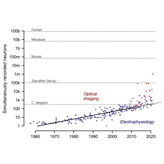
| 2011 | 📝/🔬 | “Moore’s law” of neuroscience | Stevenson and Kording predict an exponential growth of numbers of simultaneously recorded neurons every ~7 years |
| 2013 | 🔬 | Three-photon microscopy demonstrated for deep brain imaging (Horton et al.) | Extends functional imaging to deeper cortical and subcortical structures |
| 2014 | 📝 | Urbanczik–Senn dendritic predictive plasticity | Introduces plasticity driven by mismatch between somatic output and dendritic prediction |
| 2014 | 📝 | Systematic dynamical theory of spiking computation (Gerstner et al.) | Establishes a unified dynamical framework linking spikes, networks, and computation |
| 2014 | 🏅 | Nobel Prize in Physiology or Medicine awarded to O’Keefe and the Mosers | Honors the discovery of the brain’s spatial positioning system based on place and grid cells |
| 2015/2017 | 🧠 | Behavioral time scale synaptic plasticity (BTSP) experimentally described | Reveals learning rules operating over seconds, beyond classical STDP windows |
| 2017 | 🔬 | Neuropixels probes introduced | Enables simultaneous recording from thousands of neurons across multiple brain regions |
| 2018 | 📝 | Neural dynamics as variational inference (Isomura & Friston) | Explicitly links neuronal activity and plasticity to variational free energy minimization |
| 2018 | 📝 | Three factor learning rules unified in theoretical frameworks (Gerstner et al.) | Generalizes Hebbian plasticity by incorporating modulatory signals |
| 2018 | 👨💻 | Neuron version 8 with extended dynamical mechanisms | Introduces new features for simulating complex neuronal dynamics, including dendritic compartments and plasticity |
| 2019 | 👨💻 | Brian2 matures as standard teaching and research tool | Combines flexibility with code generation for efficient simulations |
| 2020 | 📝 | Bellec and colleagues introduce e-prop | Biologically motivated approximation to backpropagation through time for spiking networks |
| 2024 | 🏅 | Nobel Prize in Physics awarded to John Hopfield and Geoffrey Hinton | Honors foundational energy-based concepts underlying modern machine learning and neural network theory |
Legend:
- 🧠 Neuroscience/biological discovery
- 🔬 Experimental technique/method
- 📝 Theoretical/mathematical development
- 👨💻 Computational tool/simulator
- 🏅 Nobel Prize awarded for relevant work
This list is necessarily selective. It emphasizes developments that shaped how neural activity is modeled as a dynamical system, rather than cataloging all advances in computational neuroscience. However, if you think important milestones are missing, please let me know in the comments below.
Closing remarks
I see neural dynamics occupying a central position within the field of computational neuroscience. It provides the language in which time, change, and interaction are made explicit. While it does not define the entire field, it supplies the mathematical and conceptual tools needed to understand how neural systems evolve, stabilize, and learn.
The perspective outlined here is deliberately dynamical and model driven. It reflects an interest in equations, phase spaces, and mechanisms rather than in purely descriptive or statistical approaches. This is not meant as a value judgment, but as a clarification of scope. Computational neuroscience is broader than neural dynamics, and neural dynamics gains much of its relevance precisely because it interfaces with experiments, data analysis, and theories of computation.
This overview should therefore be read as a living document. Its purpose is to orient, not to prescribe, and to serve as a conceptual anchor for my past and future posts rather than as a definitive account of the field.
References and further reading
- Wulfram Gerstner, Werner M. Kistler, Richard Naud, and Liam Paninski, Neuronal Dynamics: From Single Neurons to Networks and Models of Cognition, 2014, Cambridge University Press, ISBN: 978-1-107-06083-8, free online version
- Hodgkin, A. L., & Huxley, A. F., A quantitative description of membrane current and its application to conduction and excitation in nerve, 1952, The Journal of Physiology, 117(4), 500–544, doi: 10.1113/jphysiol.1952.sp004764
- P. Dayan, I. F. Abbott, Theoretical Neuroscience: Computational and Mathematical Modeling of Neural Systems, 2001, MIT Press, ISBN: 0-262-04199-5
- Izhikevich, Eugene M., (2010), Dynamical systems in neuroscience: The geometry of excitability and bursting (First MIT Press paperback edition), The MIT Press, ISBN: 978-0-262-51420-0
- G. Bard Ermentrout, & David H. Terman, Mathematical Foundations of Neuroscience, 2010, Book, Springer Science & Business Media, ISBN: 9780387877082
- Christoph Börgers, An Introduction to Modeling Neuronal Dynamics, 2017 , Vol. 66, Springer International Publishing, doi: 10.1007/978-3-319-51171-9
- Gerasimos G. Rigatos, Advanced Models of Neural Networks: Nonlinear Dynamics and Stochasticity in Biological Neurons, 2015, Springer-Verlag Berlin Heidelberg, doi: 10.1007/978-3-662-43764-3
- Miller, Paul,, An introductory course in computational neuroscience, 2018, The MIT Press, ISBN: 978-0-262-34756-3
- Pezon, Schmutz, Gerstner, Linking neural manifolds to circuit structure in recurrent networks, 2024, bioRxiv 2024.02.28.582565, doi: 10.1101/2024.02.28.582565ꜛ
The list above is by no means exhaustive. It summarizes the main sources with which I would start my own exploration of neural dynamics. I highly recommend starting with Gerstner et al. (2014) for a comprehensive and mathematically rigorous introduction to the field. Also, each post in this blog contains further references and links to original articles, reviews, and textbooks that can help deepen your understanding of specific topics.


comments